Find specific cells in Excel - !SEMTools for Excel

Find cells in Excel - built-in tools vs add-in tools

Finding the right cells by a certain criterion or several is one of the most common tasks when working in Excel.

Find Cells in Excel (Built-in Tools and Functions)

Excel offers several built-in ways to locate specific cells based on their contents. These can be cells that contain a certain word, number, error, or even just be blank. Depending on the task, you can use features like Find and Replace, filters, Conditional Formatting, or logical and text functions. In this article, we’ll explore the main built-in tools in Excel that help you quickly identify which cells meet your criteria.

What Does “Find” Even Mean in Excel?

Before diving in, it’s worth pointing out that the word “find” means different things to different Excel users:

Some users want to highlight specific cells — Conditional Formatting is a great tool for this.
Others want to filter their data to only see cells that meet certain criteria — Excel’s Filter feature works well here.
Some users prefer to extract relevant cells to another location for further analysis.
Others might want to add a marker or label next to matched cells — formulas using IF can help with that.
And when comparing ranges or looking for duplicates, functions like UPPER, COUNTIF, or MATCH come into play.

But first, let’s take a moment to understand what a cell really is in Excel.

An Excel cell is more than just a value — it has three key components:

The value (what’s inside)
The formula (how it got there)
The formatting (how it looks)

That means you can find or identify cells in three main ways:

By their value
By their formula
By their format

This guide walks through how to use each approach and links to useful examples.

Finding Cells by Value

Most of the time, when people want to “find” something in Excel, they’re looking for specific values inside cells. These values can be considered individually or as part of a larger dataset.

Find Unique or Duplicate Cells

A common task is finding duplicates or unique values. For example:

A duplicate is a value that shows up more than once.
A unique value appears only once.

Excel offers a few ways to handle this, including:

Within a single range: highlight all repeated values in a column.
Between two ranges: compare two lists and highlight matching or non-matching items.
Row-by-row comparison: check if the same value appears in the same position across different rows.
Ignore order (implicit duplicates): detect phrases like “buy sofa” and “sofa buy” as duplicates.

Learn more in the guide: [How to find implicit duplicates in Excel].

Finding Cells That Contain Text

When your cells contain text, your search is usually string-based. You might want to:

Find cells that contain a certain word or substring
Find cells that contain all words from a list
Or find cells that contain at least one word from a list
Search for cells that start with or end with certain patterns

If your search involves just one condition, Find and Replace can usually do the trick. For two conditions, Advanced Filters are useful.

For more complex text matching — like multiple conditions or custom patterns — you’ll want to use formulas or tools like the !SEMTools add-in, which simplifies these tasks with pre-built procedures.

Finding Cells With Numbers

Working with numbers is a bit different — and sometimes trickier — than working with text. That’s because:

Some cells contain only numbers.
Some contain both text and numbers (e.g., “Price: 500”).
Some look like numbers but are stored as text.

If you’re working with pure numbers, you can search using comparisons:

Equals / Not equals
Greater than / Less than
Between values
Above or below average
Top or bottom N values

What about numbers inside text?

That’s where it gets tricky. You can’t apply numeric filters directly. But there are workarounds:

Use formulas to extract the number part into another column.
Use array formulas to search for numbers as text:

=COUNT(SEARCH({"2006":"2007":"2008":"2009":"2010":"2011":"2012":"2013":"2014":"2015":"2016":"2017":"2018":"2019":"2020":"2021":"2022":"2023"};A1))>0

This will return TRUE if any of the specified years are found in the cell.

Finding Cells by Formatting

Sometimes, what you’re looking for isn’t the content — it’s the format. Maybe you need to find:

All bold cells
Cells in italics
Cells with underlining
Or even those using a certain font color, fill color, or border

Excel has built-in tools (like Find & Replace > Format) for this, but they’re quite limited at some point.

how to find cells by their format in Excel

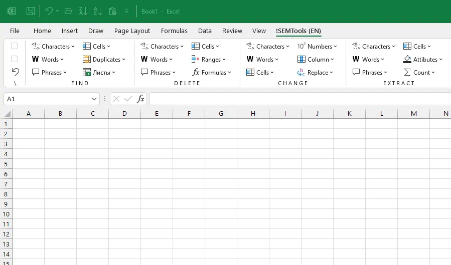
Find Cells in Excel with !SEMTools

The Find Cells section in the !SEMTools add-in helps you locate Excel cells based on their content, structure, frequency, or pattern. It’s a powerful set of tools that goes far beyond what standard Excel features can offer — saving you hours of manual work.

Find cells menu in Excel with !SEMTools add-in

Find Cells by Content

This group of tools is designed to detect whether a cell contains specific text:

Contains (from a list) — Finds all cells that contain at least one item from a list. For example, it can highlight cells with “buy”, “order”, “deal”, or “cheap”.
Starts with… — Finds cells that begin with specific patterns. You can use a custom list or built-in ones like common prepositions.
Ends with… — Similar to the above, but checks the end of the text. This is useful for spotting location or context tags at the end of phrases (e.g., “in NYC”, “for home”).
REGEX pattern match — Search cells using advanced regular expressions. Great for finding numeric patterns, specific string lengths, or things like URLs.

Find Cells by Frequency

Frequency refers to how often a value appears within a given range. This section helps distinguish whether a cell value is unique or duplicated — and where in the sequence it appears.

Unique only — Highlights cells that appear once and only once.
Duplicates only — Finds all values that repeat two or more times.
First match only — Marks only the first occurrence of each repeated value.
Last match only — Marks only the last occurrence of repeated entries.

Note: If a cell is unique, it is automatically considered both the first and last occurrence.

Find Blank Cells

This tool identifies empty cells within a selected range. It’s especially useful for data quality checks, incomplete tables, or reporting preparation.

Find Duplicates

The Find Duplicates section detects repeating values using more refined logic than Excel’s built-in tools.

Duplicates within a range:

All except first — Highlights all duplicates except the first instance.
All including first — Marks every repeated cell, including the original.
Implied duplicates — Detects phrases that use the same words in a different order (e.g., “buy sofa” vs. “sofa buy”), only marking one instance. This is extremely helpful in keyword cleanup.

Duplicates across ranges:

Exact match — Compares two ranges to find matching values.
Implied duplicates — Finds phrases that are semantically the same but written in a different word order across two data sets.

This section dramatically speeds up keyword deduplication and helps standardize datasets into unique, clean lists.

This post is also available in RU.