
You may be looking for the REPLACE function in Excel. This page is about bulk find and replace. If you only need to find cells, see how to find cells by several conditions.
When working with text data in Excel, it’s often necessary to find and replace multiple values with their corresponding alternatives. Sometimes you need to replace words with other words (e.g., synonyms), sometimes several characters with other characters.
The more such find-and-replace operations you have to perform, the more complex the task becomes—and the more important it is to know the tools that can simplify and speed up the process. Below are all the tools I know, including the ones I created myself.
Author of the !SEMTools add-in and creator of this site, Dmitry Tumaykin
Find and Replace in Excel
Find and Replace is one of the most used features in Excel. The built-in tool replaces only one value per run, but in many different ways. Let’s see how to work with it efficiently.
Keyboard shortcuts
These key combinations noticeably speed up the work:
- Open the Find dialog: Ctrl+F.
- Open the Find and Replace dialog: Ctrl+H.
- Select all found cells (after clicking Find All): Ctrl+A.
- Clear all found cells: Ctrl+Delete.
- Enter the same value in all found cells: type the text, then press Ctrl+Enter.
In the example below, I find certain cells and then edit them. Unlike replacing, editing the found cells lets you change their content entirely:

When Find and Replace doesn’t work
I’ve been stuck in this situation more than once myself. You’re sure, you see with your own eyes that the text is there, but Excel says:

or, when replacing:

The advice to click Options in both messages is actually useful: most likely, Match case or Match entire cell contents is checked, and that prevents Excel from finding the text. Excel remembers the settings of the last search, so a checkbox you used an hour ago still works against you.

Wildcards, or how to find “*”
The dry official Excel help says:
- you can use the wildcards “*” and “?”;
- “*” means any number of characters, including none, and “?” means any single character;
- they work in Find and Replace.
What it doesn’t say is that combined with Match entire cell contents, these characters let you, without the Advanced Filter or Go To Special:
- find cells that end with a certain character, word or text (“*ing”);
- find cells that start with a certain character, word or text (“buy*”);
- find non-empty cells (“*”).
In the example below, we find all two-digit numbers (“??”), then the numbers ending and starting with 7 (“*7” and “7*”), and finally all non-empty cells. Remember that Ctrl+A selects all found results.
So how do you find the asterisk itself? Right, I almost forgot. To find “*”, type a tilde before it: “~*”. The tilde is usually under the Esc key. It escapes the asterisk and the question mark, so Excel doesn’t treat them as wildcards.
Replace multiple values with multiple values
Bulk replacement in Excel is a common need: quickly replace several characters, words and so on with others. Yet there is still no simple tool for it in standard Excel.
Still, if you really need it, any task can be solved. Depending on what you replace, combinations of functions, regular expressions or, in the hardest cases, the !SEMTools add-in will help.
Oddly enough, the REPLACE function doesn’t fit here: it requires the exact position of the text to replace. The SUBSTITUTE function does.
Bulk replacement with nested SUBSTITUTE
By nesting several SUBSTITUTE functions in one formula, you can replace several values at once. Excel allows up to 64 nesting levels, so there is plenty of room. For example, here is how to turn text into “leet speak”:
=SUBSTITUTE(SUBSTITUTE(SUBSTITUTE(SUBSTITUTE(SUBSTITUTE(SUBSTITUTE(SUBSTITUTE(A1,"A","4"),"E","3"),"G","6"),"I","1"),"O","0"),"S","5"),"T","7")
| A | B | |
|---|---|---|
| 1 | Text | Result |
| 2 | GOOD GAME | 600D 64M3=SUBSTITUTE(SUBSTITUTE(SUBSTITUTE(SUBSTITUTE(SUBSTITUTE(SUBSTITUTE(SUBSTITUTE(A2,"A","4"),"E","3"),"G","6"),"I","1"),"O","0"),"S","5"),"T","7") |
| 3 | SEMTOOLS | 53M700L5=SUBSTITUTE(SUBSTITUTE(SUBSTITUTE(SUBSTITUTE(SUBSTITUTE(SUBSTITUTE(SUBSTITUTE(A3,"A","4"),"E","3"),"G","6"),"I","1"),"O","0"),"S","5"),"T","7") |
| 4 | Excel tips | 3xcel tips=SUBSTITUTE(SUBSTITUTE(SUBSTITUTE(SUBSTITUTE(SUBSTITUTE(SUBSTITUTE(SUBSTITUTE(A4,"A","4"),"E","3"),"G","6"),"I","1"),"O","0"),"S","5"),"T","7") |
Each SUBSTITUTE replaces one letter and passes the result to the next. Case matters: in “Excel tips” only uppercase letters would be replaced, and there are none except E.

But this solution has its drawbacks:
- SUBSTITUTE is case-sensitive, so to replace a letter you have to list both its uppercase and lowercase versions. In some cases, like the one above, this is an advantage.
- A maximum of 64 replacements. That’s a lot, but still a limit.
- The replacement is bulk only formally: the formula has to be typed, filled down the column, pasted as values and the helper column deleted. And every new rule means editing a long formula.
Template formula for multiple replacements
Instead of writing the patterns into the formula, you can refer to cells where you type the rules. This saves time, because you don’t need to edit a complex formula.
The formula below replaces the text in cell D1 by the rules in A1:B64: each value in column A is replaced with the value next to it in column B. You can paste it into any cell outside A1:B64. Empty rows in the rules table don’t break it: SUBSTITUTE with an empty search value simply returns the text unchanged. Triple-click the formula to select it entirely:
=SUBSTITUTE(SUBSTITUTE(SUBSTITUTE(SUBSTITUTE(SUBSTITUTE(SUBSTITUTE(SUBSTITUTE(SUBSTITUTE(SUBSTITUTE(SUBSTITUTE(SUBSTITUTE(SUBSTITUTE(SUBSTITUTE(SUBSTITUTE(SUBSTITUTE(SUBSTITUTE(SUBSTITUTE(SUBSTITUTE(SUBSTITUTE(SUBSTITUTE(SUBSTITUTE(SUBSTITUTE(SUBSTITUTE(SUBSTITUTE(SUBSTITUTE(SUBSTITUTE(SUBSTITUTE(SUBSTITUTE(SUBSTITUTE(SUBSTITUTE(SUBSTITUTE(SUBSTITUTE(SUBSTITUTE(SUBSTITUTE(SUBSTITUTE(SUBSTITUTE(SUBSTITUTE(SUBSTITUTE(SUBSTITUTE(SUBSTITUTE(SUBSTITUTE(SUBSTITUTE(SUBSTITUTE(SUBSTITUTE(SUBSTITUTE(SUBSTITUTE(SUBSTITUTE(SUBSTITUTE(SUBSTITUTE(SUBSTITUTE(SUBSTITUTE(SUBSTITUTE(SUBSTITUTE(SUBSTITUTE(SUBSTITUTE(SUBSTITUTE(SUBSTITUTE(SUBSTITUTE(SUBSTITUTE(SUBSTITUTE(SUBSTITUTE(SUBSTITUTE(SUBSTITUTE(SUBSTITUTE(D1,$A$1,$B$1),$A$2,$B$2),$A$3,$B$3),$A$4,$B$4),$A$5,$B$5),$A$6,$B$6),$A$7,$B$7),$A$8,$B$8),$A$9,$B$9),$A$10,$B$10),$A$11,$B$11),$A$12,$B$12),$A$13,$B$13),$A$14,$B$14),$A$15,$B$15),$A$16,$B$16),$A$17,$B$17),$A$18,$B$18),$A$19,$B$19),$A$20,$B$20),$A$21,$B$21),$A$22,$B$22),$A$23,$B$23),$A$24,$B$24),$A$25,$B$25),$A$26,$B$26),$A$27,$B$27),$A$28,$B$28),$A$29,$B$29),$A$30,$B$30),$A$31,$B$31),$A$32,$B$32),$A$33,$B$33),$A$34,$B$34),$A$35,$B$35),$A$36,$B$36),$A$37,$B$37),$A$38,$B$38),$A$39,$B$39),$A$40,$B$40),$A$41,$B$41),$A$42,$B$42),$A$43,$B$43),$A$44,$B$44),$A$45,$B$45),$A$46,$B$46),$A$47,$B$47),$A$48,$B$48),$A$49,$B$49),$A$50,$B$50),$A$51,$B$51),$A$52,$B$52),$A$53,$B$53),$A$54,$B$54),$A$55,$B$55),$A$56,$B$56),$A$57,$B$57),$A$58,$B$58),$A$59,$B$59),$A$60,$B$60),$A$61,$B$61),$A$62,$B$62),$A$63,$B$63),$A$64,$B$64)
In Excel 365, the same can be written much shorter with REDUCE and LAMBDA. The formula goes through the rules one by one and applies each of them to the result of the previous one:
=REDUCE(D1,SEQUENCE(ROWS($A$1:$A$64)),LAMBDA(t,i,IF(INDEX($A$1:$A$64,i)="",t,SUBSTITUTE(t,INDEX($A$1:$A$64,i),INDEX($B$1:$B$64,i)))))
| A | B | C | D | E | |
|---|---|---|---|---|---|
| 1 | Find | Replace with | Text | Result | |
| 2 | St. | Street | 12 Pine St. | 12 Pine Street=REDUCE(D2,SEQUENCE(ROWS($A$2:$A$4)),LAMBDA(t,n,IF(INDEX($A$2:$A$4,n)="",t,SUBSTITUTE(t,INDEX($A$2:$A$4,n),INDEX($B$2:$B$4,n))))) | |
| 3 | Ave. | Avenue | 5 Oak Ave., 7 Elm Rd. | 5 Oak Avenue, 7 Elm Road=REDUCE(D3,SEQUENCE(ROWS($A$2:$A$4)),LAMBDA(t,n,IF(INDEX($A$2:$A$4,n)="",t,SUBSTITUTE(t,INDEX($A$2:$A$4,n),INDEX($B$2:$B$4,n))))) | |
| 4 | Rd. | Road | Main Square | Main Square=REDUCE(D4,SEQUENCE(ROWS($A$2:$A$4)),LAMBDA(t,n,IF(INDEX($A$2:$A$4,n)="",t,SUBSTITUTE(t,INDEX($A$2:$A$4,n),INDEX($B$2:$B$4,n))))) |
The rules live in A:B — add a pair and the formula picks it up. REDUCE takes the text and applies the rules one by one to the result of the previous step. Excel 365 only; for older versions use the nested SUBSTITUTE template above.
Replace multiple values with one
With the SUBSTITUTE function
When you replace several values with the same one, the formula works the same way as above. The third argument (what to replace with) is just the same on every nesting level. By the way, if you leave it empty, two quotes with nothing between them, the formula deletes the characters. For example, all digits:
=SUBSTITUTE(SUBSTITUTE(SUBSTITUTE(SUBSTITUTE(SUBSTITUTE(SUBSTITUTE(SUBSTITUTE(SUBSTITUTE(SUBSTITUTE(SUBSTITUTE(A1,"1",""),"2",""),"3",""),"4",""),"5",""),"6",""),"7",""),"8",""),"9",""),"0","")
| A | B | |
|---|---|---|
| 1 | Text | Result |
| 2 | Order 4512 from 10/22 | Order from /=SUBSTITUTE(SUBSTITUTE(SUBSTITUTE(SUBSTITUTE(SUBSTITUTE(SUBSTITUTE(SUBSTITUTE(SUBSTITUTE(SUBSTITUTE(SUBSTITUTE(A2,"1",""),"2",""),"3",""),"4",""),"5",""),"6",""),"7",""),"8",""),"9",""),"0","") |
| 3 | Model X200 | Model X=SUBSTITUTE(SUBSTITUTE(SUBSTITUTE(SUBSTITUTE(SUBSTITUTE(SUBSTITUTE(SUBSTITUTE(SUBSTITUTE(SUBSTITUTE(SUBSTITUTE(A3,"1",""),"2",""),"3",""),"4",""),"5",""),"6",""),"7",""),"8",""),"9",""),"0","") |
The replacement is the same empty string on every level, so all ten digits disappear. A shorter way is a regex: =REGEXREPLACE(A2,"\d","").
There are simpler ways for this particular task, see how to remove numbers from cells. And to keep only letters and digits, see how to remove punctuation in Excel.
With regular expressions
Important: before Excel 365, regular expressions were not available in Excel out of the box, but the formulas below are available for free with the !SEMTools add-in. In Excel 365, the built-in REGEXREPLACE works the same way.
Regex is the most convenient solution when you need to replace several characters with one. List all of them without any separators inside square brackets, or use a ready-made class. Examples:
=REGEXREPLACE(A1,"\d","#")
=REGEXREPLACE(A1,"[A-Z]","#")
=REGEXREPLACE(A1,"[aeiou]","*")
=REGEXREPLACE(A1,"\s","_")
| A | B | C | D | E | |
|---|---|---|---|---|---|
| 1 | Pattern | Replacement | Result | Text | Order A-1024 shipped to Main St |
| 2 | \d | # | Order A-#### shipped to Main St=REGEXREPLACE($E$1,A2,B2) | ||
| 3 | [A-Z] | # | #rder #-1024 shipped to #ain #t=REGEXREPLACE($E$1,A3,B3) | ||
| 4 | [aeiou] | * | Ord*r A-1024 sh*pp*d t* M**n St=REGEXREPLACE($E$1,A4,B4) | ||
| 5 | \s | _ | Order_A-1024_shipped_to_Main_St=REGEXREPLACE($E$1,A5,B5) |
The source text is in E1 (D1 is its label); each row applies one pattern. In Excel 365 this is the built-in REGEXREPLACE; in older versions the function with the same name comes with the free !SEMTools add-in.
The first one replaces all digits with “#”, the second one all uppercase English letters, the third one all lowercase vowels. The fourth one replaces any whitespace, including tabs and line breaks, with an underscore.
If you need to replace not single characters but several values that consist of several letters, digits or symbols, use parentheses and the vertical bar “|” as a separator: =REGEXREPLACE(A1,"\s*(Inc|LLC|Ltd)\.?$","") removes any of these company suffixes at the end of a cell.
Bulk replacement in !SEMTools
The !SEMTools add-in for Excel does replacements at every level in a couple of clicks:
- characters and their combinations;
- regular expression patterns;
- whole words;
- entire cells (to some extent, an analog of the VLOOKUP function).

The procedures change the source range directly, which saves time: no formulas to remember, type in and fill down, no helper columns. All you need is to select the range, choose the procedure and point to the two columns with the “find” and “replace with” values. If you know what to replace with what, you most likely already have such lists.
Example: character replacement by occurrence
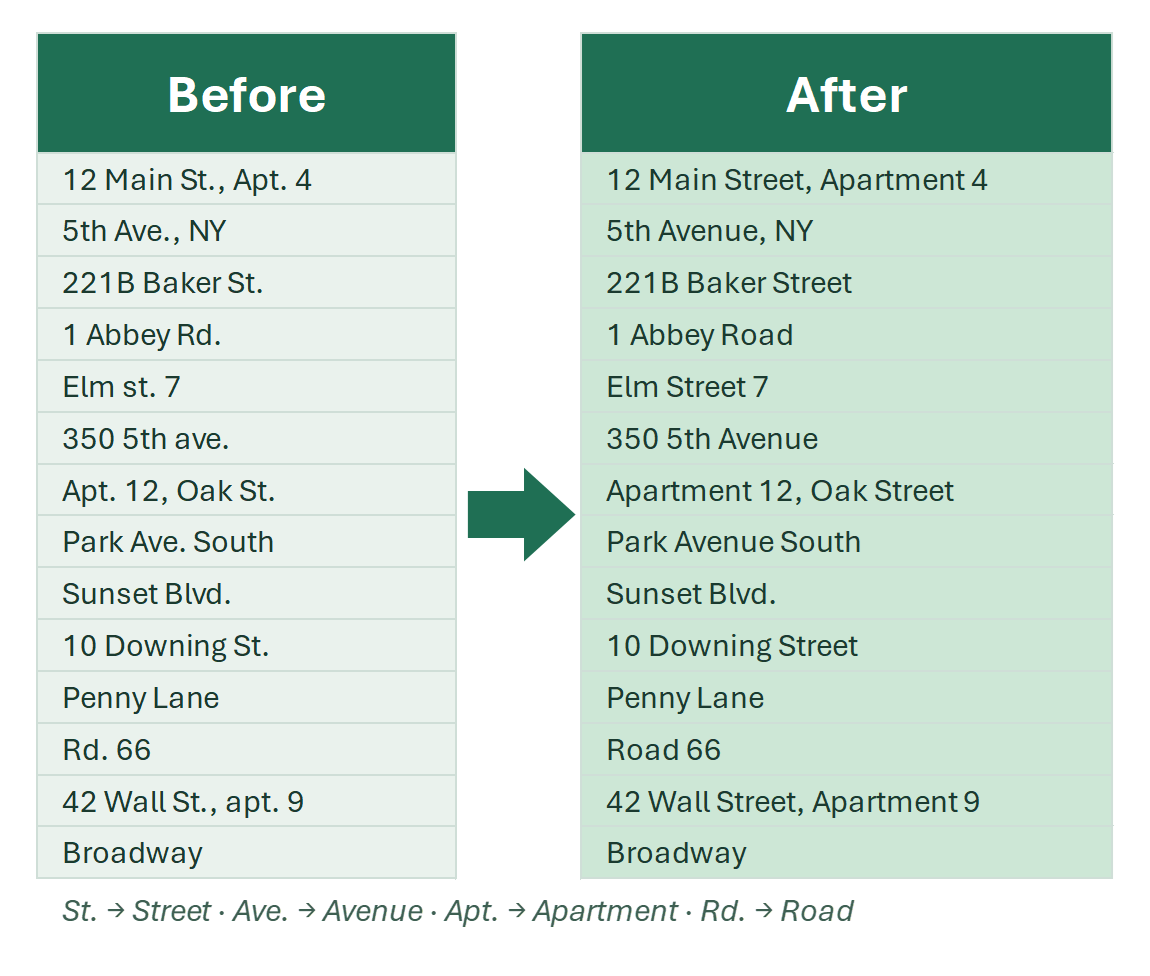
This is an analog of the regular Find and Replace, case-insensitive, by occurrence. With one difference: the replacement is bulk, and you can select as many rows with “find → replace” pairs as you need.
Below is an example with single characters, but the patterns can be anything your task requires:

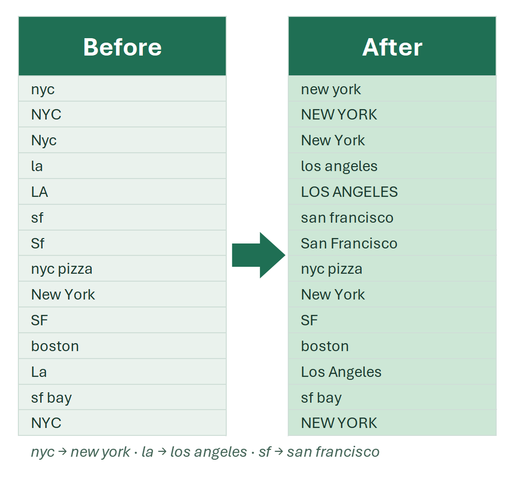
Example: replacing a list of words with another list
Simple substring search is not always good for words and phrases, because it can damage your data: replacing “cat” would also change “category”. To keep the words safe, I added procedures that replace whole words and phrases only:

A typical case is normalizing different phrases: replace all model names, sizes or brand variations with one word, and then count the unique phrases in the column to see the most popular combinations.
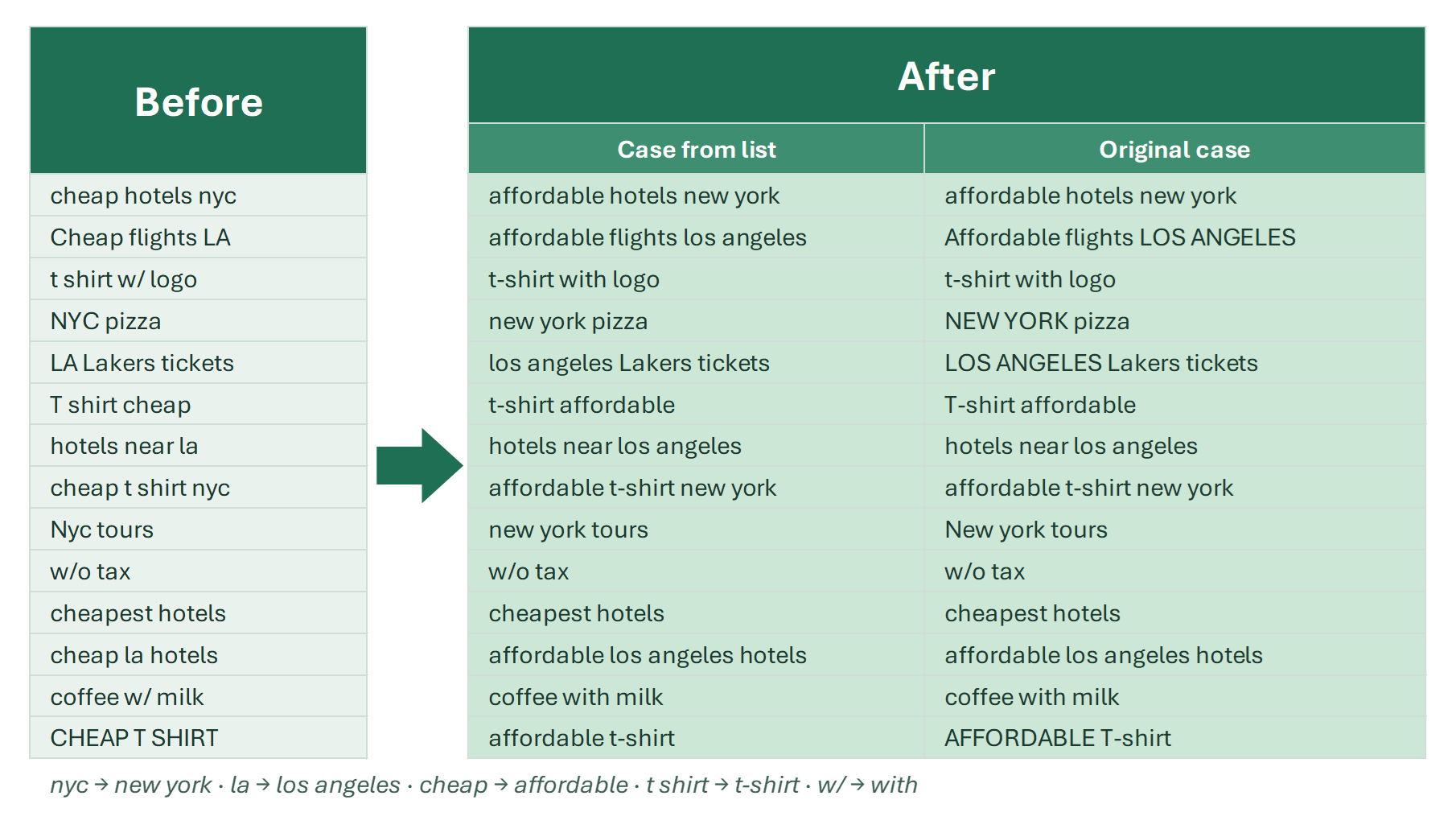
Since !SEMTools 9.18.18, there is an option to ignore punctuation in the source sentences when replacing a list of words, and the case of the words is now preserved.
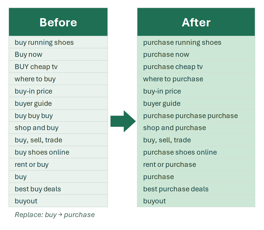
The tools are in CHANGE → Replace: Multiple replacement for substrings, Full words and phrases (Word by word, List by list), Replace full cell contents and By RegExp (first or all occurrences). Word replacement is also duplicated in CHANGE → Words → Replace.
See also:
Replace lists of characters, words or entire cells with other lists right in the source cells, without 64-level formulas or helper columns.
!SEMTools solves this and hundreds of other tasks in a couple of clicks!
Summary: which bulk replace method to choose
I hope you found what you were looking for on this page and were able to replace multiple values at once. For a single value, Find and Replace is enough, as long as you check the Options. For a few replacements, nested SUBSTITUTE works, and regex is best for sets of characters. But as soon as the rules become a list, the formula turns into a monster that has to be maintained, filled down and pasted as values. !SEMTools does the same right in place, with the rules in two columns.
You may also be interested in related operations on search and replace in Excel: