| Function category | Logical functions |
| Volatility | Non-volatile |
| Similar functions | IFERROR, ISERR, ISERROR, ISNA |
What does this function do?
The function checks the truthfulness of the first argument – a calculation or cell value. Depending on the result, calculations will be performed or other values returned.
Syntax
=IF(condition, value_if_true, value_if_false)
The condition is typically a calculation that returns a boolean result (TRUE or FALSE).
Comparison criteria commonly used: ‘=’ (equal to), ‘>’ (greater than), ‘<‘ (less than), ‘<>’ (not equal to), ‘>=’ (greater than or equal to), ‘<=’ (less than or equal to). You can compare logical, numeric, and text values with each other.
The function can also accept numbers as input. Numbers not equal to zero are considered equivalent to TRUE, 0 to FALSE.
Other features of the IF function:
- If the input value is given as an array, the IF function will process each element of that array.
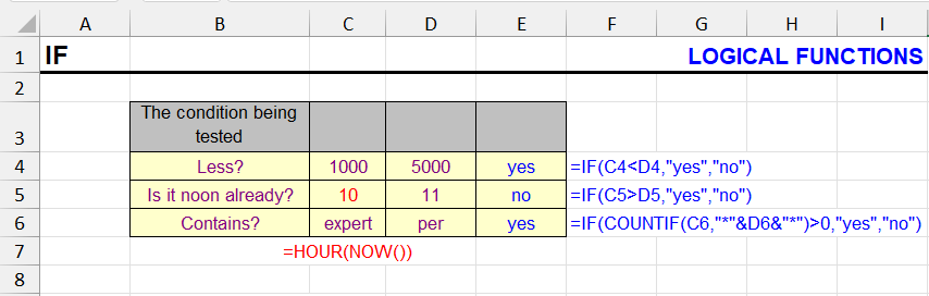
Usage examples
Example 1
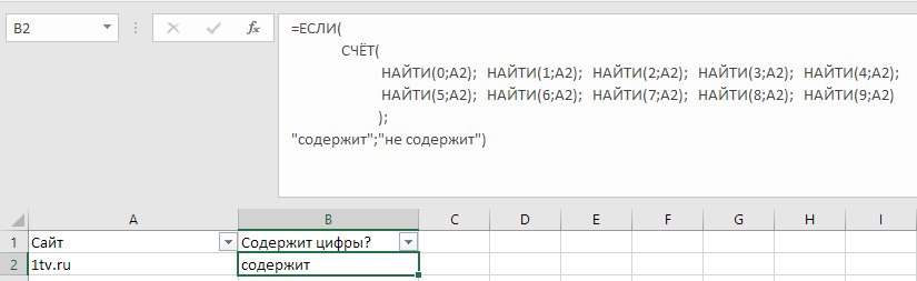
How to check if a cell contains numbers? This site has a detailed discussion of solving this task, including using the !SEMTools add-in, which provides the fastest solution. But now we’ll look at it using IF.
You can check if it contains each of the digits, one by one, and if it doesn’t contain any, report that it doesn’t contain any. The general pseudo-syntax for checking the truth of multiple values would involve nesting the OR function.
=IF(COUNT(check1, check2, ...), value_if_true, value_if_false)
Here COUNT will return a positive number if at least one of the expressions given to it as input (in parentheses after it) is not equal to zero or error, or 0 if none. And the IF function will treat this result as TRUE if the number is positive, and as FALSE if it equals zero.
To check for the presence of digits in a string, we’ll use the SEARCH function.
Let’s try to apply the syntax to the example with digits. This is what the formula will look like (don’t be surprised by line breaks and spaces – they are ignored in Excel and you can compose complex formulas similarly for convenience).
Example 2
How to speed up VLOOKUP by 50,000 times? Using IF and a second VLOOKUP! No, there’s no mistake here. You can read in detail about this fascinating phenomenon in the corresponding article about the VLOOKUP function, and here we’ll just provide the file and formula involving IF.
This is what its syntax looks like:
=IF(VLOOKUP(A1, $E$1:$E$400000, 1, 1)=A1, VLOOKUP(A1, $E$1:$F$400000, 2, 1), "")
In human language, the formula means that if the value returned by binary search in the first column equals the search value, we perform a second binary search – returning the second column. If not – return an empty string.
Example 3
Excel versions before 2016 lack the MAXIFS and MINIFS functions. But nothing prevents us from creating their equivalent using array formulas.
Let’s say we want to calculate the largest and smallest even number in range A1:A10.
We’ll use the ISEVEN function (appeared in Excel 2007) on the array and return the number itself if it’s even, and an empty string if it’s odd. We’ll process the resulting array with MAX and MIN functions:
Largest even number in the range:
={MAX(IF(ISEVEN(A1:A10+0), A1:A10, ""))}
Smallest even number in the range:
={MIN(IF(ISEVEN(A1:A10+0), A1:A10, ""))}
And if we have Excel 2003 and the ISEVEN function is also unavailable, we use the MOD function, checking the remainder when divided by 2:
Smallest even number in the range (Excel 2003)
={MAX(IF(MOD(A1:A10, 2)=0, A1:A10, ""))}
Largest even number in the range (Excel 2003)
={MIN(IF(MOD(A1:A10, 2)=0, A1:A10, ""))}
Multiple nested IF functions
Sometimes one IF is not enough. For example, you need to check several options and show a different result for each. In such cases, several nested IF functions are used – one inside another. This is convenient when you need to select text or a value depending on multiple conditions.
For example, the following formula can be used in an Excel document where you automatically substitute the correct declension of the phrase “calendar day” depending on the number of days – for example, in a vacation request or memo.
Example scenario:
An employee fills out a vacation request and in cell M7 specifies the number of days (e.g., 3, 5, 14, etc.).
In English, the word “day” changes depending on the number:
- 1 → calendar day
- 2+ → calendar days
=IF(M7=1, "calendar day", "calendar days")
This formula automatically generates the correct phrase based on the number of days:
- if M7 = 1 → “calendar day”
- if M7 = 2, 3, 4, 5, etc. → “calendar days”
This phrase can then be used in the request text using concatenation (CONCAT, CONCATENATE or with the ampersand “&”).
This eliminates manual text correction in requests and other documents where it’s important to follow English grammar rules for numerical declension.
When you have too many IF functions
If you use several nested IF functions, the formula becomes long and inconvenient:
=IF(A1=1, "One", IF(A1=2, "Two", IF(A1=3, "Three", "Other")))Alternatives to nested IF functions, such as VLOOKUP and CHOOSE, help make formulas simpler, clearer, and easier to edit.
✅ Why use the CHOOSE function
If A1 is simply a number (e.g., 1, 2, 3), the formula can be simplified:
=CHOOSE(A1, "One", "Two", "Three", "Four")If A1 = 3, the result will be “Three”.
🔍 Why use VLOOKUP
If you have a lookup table:
| Value | Result |
|---|---|
| 1 | One |
| 2 | Two |
| 3 | Three |
| 4 | Four |
You can use VLOOKUP (vertical lookup in a table):
=VLOOKUP(A1, A2:B5, 2, 0)This is especially convenient when you want to change values directly in the table, not in the formula itself.
🧠 Conclusion
- IF — good for 2-3 conditions
- CHOOSE — ideal if you have a sequential number
- VLOOKUP — convenient when values are stored in a table
Other Logical functions in Excel
IF, AND, OR, NOT, IFERROR, IFS, SWITCH, CHOOSE
Like the article? Help its author! Buy !SEMTools, it has lots of useful instruments to process text data.