| Function category | Text functions |
| Volatility | Non-volatile |
| Similar functions | DATEVALUE — converts text to date |
| Similar procedures | Convert numbers stored as text to actual numbers |
What does the VALUE function do?
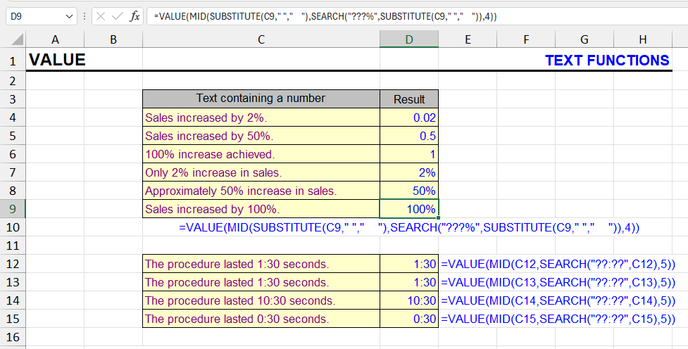
This function converts a piece of text that resembles a number into an actual number.
If the number is in the middle of a long text fragment, it will need to be extracted using other text functions such as SEARCH, MID, FIND, REPLACE, LEFT, RIGHT.
VALUE function syntax
=VALUE(text)
| A | B | C | |
|---|---|---|---|
| 1 | Text in cell | =VALUE(A) | Comment |
| 2 | 123 | 123=VALUE(A2) | plain number |
| 3 | 1,250.50 | 1250.5=VALUE(A3) | thousands separator |
| 4 | 42 | 42=VALUE(A4) | spaces at the edges are ignored |
| 5 | -7.5 | -7.5=VALUE(A5) | negative with a decimal point |
| 6 | 1.250,5 | #VALUE!=VALUE(A6) | European format isn’t a number in US settings |
| 7 | abc | #VALUE!=VALUE(A7) | doesn’t look like a number |
Cells in column A are text (aligned left), the result is a number. The decimal and thousands separators must match your Windows regional settings. For other formats use NUMBERVALUE: =NUMBERVALUE(A6,",",".").
VALUE: result and input format
No special formatting required.
The result will be displayed as a numeric value based on the source text.
If the % sign is included in the text, the result will be a decimal that can then be formatted as a percentage.
If the source text format appears as time hh:mm, the result will be time.
The same applies to other formats.
| A | B | C | |
|---|---|---|---|
| 1 | Text | VALUE result | With formatting |
| 2 | 15% | 0.15=VALUE(A2) | 15% |
| 3 | 12.5% | 0.125=VALUE(A3) | 12.5% |
| 4 | 12:30 | 0.520833333=VALUE(A4) | 12:30 |
| 5 | 3/1/2026 | 46082=VALUE(A5) | 3/1/2026 |
Excel stores percentages as fractions, times as a part of a day, and dates as day numbers since 1900. VALUE returns the raw number, and cell formatting gives it the familiar look.
VALUE formula example
Extracting percentage values from text is difficult without knowing in advance how many digits it contains. This can range from 1 digit (5%) to 4 digits with a decimal (12.25%).
The only way to identify the percentage value is that it always ends with the % sign. It's impossible to determine the beginning of the value except that it's preceded by a space.
The main problem is calculating the length of the number to extract it.
If during extraction we assume a maximum length of four digits and the % sign, when the percentage is only one digit, regular extraction using the mask "?????%" will include letters in the expression.
To work around this problem, you can use the SUBSTITUTE function to increase the number of spaces between words in the text. Now when extracting using the mask:
?????%any extra characters will be spaces, which the VALUE function will ignore.
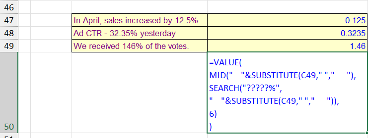
The formula below is similar to the one in the picture and will extract percentages from cell A1 with lengths from 1 to 5 characters, including decimal point:
=VALUE(MID(REPT(" ",5)&SUBSTITUTE(A1," ",REPT(" ",5)),SEARCH("?????%",REPT(" ",5)&SUBSTITUTE(A1," ",REPT(" ",5))),6))
| A | B | |
|---|---|---|
| 1 | Text | Percent |
| 2 | Sales grew 12.5% last year | 0.125=VALUE(MID(REPT(" ",5)&SUBSTITUTE(A2," ",REPT(" ",5)),SEARCH("?????%",REPT(" ",5)&SUBSTITUTE(A2," ",REPT(" ",5))),6)) |
| 3 | 7% off everything | 0.07=VALUE(MID(REPT(" ",5)&SUBSTITUTE(A3," ",REPT(" ",5)),SEARCH("?????%",REPT(" ",5)&SUBSTITUTE(A3," ",REPT(" ",5))),6)) |
| 4 | Conversion reached 100% by March | 1=VALUE(MID(REPT(" ",5)&SUBSTITUTE(A4," ",REPT(" ",5)),SEARCH("?????%",REPT(" ",5)&SUBSTITUTE(A4," ",REPT(" ",5))),6)) |
| 5 | Rate 0.25% per year | 0.0025=VALUE(MID(REPT(" ",5)&SUBSTITUTE(A5," ",REPT(" ",5)),SEARCH("?????%",REPT(" ",5)&SUBSTITUTE(A5," ",REPT(" ",5))),6)) |
Every space is replaced with five, so there is always a “buffer” of spaces before the number, and the 6-character window ending in % captures a number of 1 to 5 characters. VALUE drops the spaces and turns “12.5%” into 0.125. The previous version of the formula had lost its spaces when published — fixed.
How the VALUE function helps work with numbers in text
The VALUE function in Excel converts text to numbers when possible. This is especially useful when data is presented as text (e.g., "123", "005", "1,000"), but you need to perform arithmetic operations — addition, multiplication, percentage, etc. Without prior conversion, Excel won't recognize such values as numbers, and the formula result will be incorrect or return an error.
VALUE is often combined with text functions RIGHT, LEFT, MID and SEARCH. This allows you to "cut out" the needed part of a string and then apply mathematical operations to it. This approach is especially relevant when processing codes, SKUs, prices, identifiers that are stored as text.
Useful formulas with VALUE function
1. Round percentages inside a text string:
=TRIM(REPLACE(SUBSTITUTE(A1," ",REPT(" ",10)),MIN(IFERROR(SEARCH(CHAR(ROW(48:57)),SUBSTITUTE(A1," ",REPT(" ",10))),"")),6,TEXT(ROUND(VALUE(MID(SUBSTITUTE(A1," ",REPT(" ",10)),MIN(IFERROR(SEARCH(CHAR(ROW(48:57)),SUBSTITUTE(A1," ",REPT(" ",10))),"")),6)),2),"0%")))| A | B | |
|---|---|---|
| 1 | Original string | Result |
| 2 | 81.87% of users prefer dark mode | 82% of users prefer dark mode=TRIM(REPLACE(SUBSTITUTE(A2," ",REPT(" ",10)),MIN(IFERROR(SEARCH(CHAR(ROW(48:57)),SUBSTITUTE(A2," ",REPT(" ",10))),"")),6,TEXT(ROUND(VALUE(MID(SUBSTITUTE(A2," ",REPT(" ",10)),MIN(IFERROR(SEARCH(CHAR(ROW(48:57)),SUBSTITUTE(A2," ",REPT(" ",10))),"")),6)),2),"0%"))) |
| 3 | Market share 34.21% in 2025 | Market share 34% in 2025=TRIM(REPLACE(SUBSTITUTE(A3," ",REPT(" ",10)),MIN(IFERROR(SEARCH(CHAR(ROW(48:57)),SUBSTITUTE(A3," ",REPT(" ",10))),"")),6,TEXT(ROUND(VALUE(MID(SUBSTITUTE(A3," ",REPT(" ",10)),MIN(IFERROR(SEARCH(CHAR(ROW(48:57)),SUBSTITUTE(A3," ",REPT(" ",10))),"")),6)),2),"0%"))) |
MIN(SEARCH(CHAR(48…57))) finds the first digit, MID cuts 6 characters of the percentage, VALUE turns them into a fraction, ROUND to 2 digits gives a whole percent, and TEXT with "0%" puts it back into the string. In Excel 2019 and earlier enter it with Ctrl+Shift+Enter.
For example, the string “81.87% of users prefer dark mode” becomes “82% of users prefer dark mode”.
2. Extract the first number and calculate 20% VAT:
="VAT: "&TEXT(VALUE(MID(SUBSTITUTE(A1," ",REPT(" ",10)),MIN(IFERROR(SEARCH(CHAR(ROW(48:57)),SUBSTITUTE(A1," ",REPT(" ",10))),"")),9)/5,"0")&" USD"
| A | B | |
|---|---|---|
| 1 | String | VAT 20% |
| 2 | Product cost - 225,500 USD | VAT: 45100 USD="VAT: "&TEXT(VALUE(MID(SUBSTITUTE(A2," ",REPT(" ",10)),MIN(IFERROR(SEARCH(CHAR(ROW(48:57)),SUBSTITUTE(A2," ",REPT(" ",10))),"")),9)/5,"0")&" USD" |
| 3 | Price 1500 USD before tax | VAT: 300 USD="VAT: "&TEXT(VALUE(MID(SUBSTITUTE(A3," ",REPT(" ",10)),MIN(IFERROR(SEARCH(CHAR(ROW(48:57)),SUBSTITUTE(A3," ",REPT(" ",10))),"")),9)/5,"0")&" USD" |
MID cuts up to 9 characters starting at the first digit; the extra characters are spaces, which VALUE ignores. With US settings “225,500” is read as 225500. Dividing by 5 gives 20% of a pre-tax amount; if VAT is already included, divide by 6.
If A1 = "Product cost - 225,500 USD", result: VAT: 45100 USD
3. Add 5 to the number at the beginning of text
For values like "30 cm".
=TRIM(REPLACE(SUBSTITUTE(A1," ",REPT(" ",2)),1,3,TEXT(VALUE(LEFT(SUBSTITUTE(A1," ",REPT(" ",2)),3))+5,"0")&" "))| A | B | |
|---|---|---|
| 1 | Original | +5 |
| 2 | 30 cm | 35 cm=TRIM(REPLACE(SUBSTITUTE(A2," ",REPT(" ",2)),1,3,TEXT(VALUE(LEFT(SUBSTITUTE(A2," ",REPT(" ",2)),3))+5,"0")&" ")) |
| 3 | 7 pcs | 12 pcs=TRIM(REPLACE(SUBSTITUTE(A3," ",REPT(" ",2)),1,3,TEXT(VALUE(LEFT(SUBSTITUTE(A3," ",REPT(" ",2)),3))+5,"0")&" ")) |
| 4 | 95 kg | 100 kg=TRIM(REPLACE(SUBSTITUTE(A4," ",REPT(" ",2)),1,3,TEXT(VALUE(LEFT(SUBSTITUTE(A4," ",REPT(" ",2)),3))+5,"0")&" ")) |
Double spaces make LEFT(…,3) grab a 1–2 digit number with spaces, and VALUE drops them. For numbers of three or more digits increase REPT and the LEFT length.
If A1 = "30 cm", result: 35 cm
4. Increase the number at the end of text by 15%:
=REPLACE(A1,LEN(A1)-2,3,TEXT(VALUE(RIGHT(A1,3))*1.15,"0"))| A | B | |
|---|---|---|
| 1 | Original | +15% |
| 2 | Amount045 | Amount52=REPLACE(A2,LEN(A2)-2,3,TEXT(VALUE(RIGHT(A2,3))*1.15,"0")) |
| 3 | Code200 | Code230=REPLACE(A3,LEN(A3)-2,3,TEXT(VALUE(RIGHT(A3,3))*1.15,"0")) |
| 4 | Lot100 | Lot115=REPLACE(A4,LEN(A4)-2,3,TEXT(VALUE(RIGHT(A4,3))*1.15,"0")) |
RIGHT takes the last three digits, VALUE turns them into a number (045 → 45), the result is rounded with the "0" format and put in place of the old digits. 45 × 1.15 = 51.75, so the result is Amount52, not Amount052 as the article said before — fixed.
If A1 = "Amount045", result: Amount52
Other Text functions in Excel
DATEVALUE, TEXT, LEFT, RIGHT, MID, FIND, SEARCH, REPLACE, SUBSTITUTE, TRIM, LEN
See also:
Like the article? Help its author! Buy !SEMTools, it has lots of useful instruments to process text data.