
| Function category | Logical functions |
| Volatility | Non-volatile |
| Similar functions | OR — checks if any condition is true NOT — reverses logical value IF — performs conditional calculations |
What does the AND function do?
The AND function checks whether all provided conditions are TRUE. Returns TRUE only if every condition is met, FALSE if any condition is not met.
It can be used to verify that a series of numbers meets specific conditions, or to check that a number or date falls between upper and lower limits.
Like the OR function, it's typically used in combination with other logical functions, most commonly with the IF function, and with array formulas.
AND function syntax
=AND(logical1, [logical2], ...)=AND(value_range)| A | B | C | D | E | |
|---|---|---|---|---|---|
| 1 | Value 1 | Value 2 | Value 3 | AND | AND(range) |
| 2 | TRUE | TRUE | TRUE | TRUE=AND(A2,B2,C2) | TRUE=AND(A2:C2) |
| 3 | TRUE | FALSE | TRUE | FALSE=AND(A3,B3,C3) | FALSE=AND(A3:C3) |
| 4 | 1 | 5 | text | TRUE=AND(A4:C4) | TRUE=AND(A4:C4) |
| 5 | 0 | TRUE | TRUE | FALSE=AND(A5,B5,C5) | FALSE=AND(A5:C5) |
| 6 | text | #VALUE!=AND(A6:C6) | #VALUE!=AND(A6:C6) |
Any number except 0 counts as TRUE, 0 as FALSE. Text and empty cells inside a range are skipped; if nothing else is left, AND returns #VALUE!.
AND: result and input format
The function correctly processes:
- Numbers and calculations returning numbers
- Logical expressions (TRUE, FALSE) and calculations returning them
- Cells containing these values
- Cell ranges where at least one cell contains numbers or logical values
- Arrays of values or calculations
If a range containing text values is provided, they are ignored by the function, as are empty cells.
The function returns an error if:
- only text or empty cells are provided as input (one or more)
- there are errors among the values (#VALUE!, #N/A, #NAME?, #NULL!, #DIV/0!, #REF!, #NUM!)
AND formula examples
Example 1
The following example shows a list of test results.
The teacher wants to find students who scored above average on all three exams.
The AND function was used to verify that the score for each subject is above average.
The result TRUE is shown for students who scored above average in all three exams.
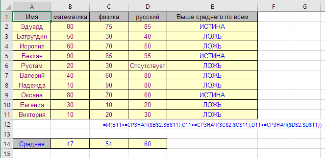
=AND(B2>=AVERAGE($B$2:$B$11),C2>=AVERAGE($C$2:$C$11),D2>=AVERAGE($D$2:$D$11))| A | B | C | D | E | |
|---|---|---|---|---|---|
| 1 | Student | Math | Physics | English | All above average? |
| 2 | Ann | 82 | 75 | 90 | FALSE=AND(B2>=AVERAGE($B$2:$B$6),C2>=AVERAGE($C$2:$C$6),D2>=AVERAGE($D$2:$D$6)) |
| 3 | Bob | 60 | 88 | 70 | FALSE=AND(B3>=AVERAGE($B$2:$B$6),C3>=AVERAGE($C$2:$C$6),D3>=AVERAGE($D$2:$D$6)) |
| 4 | Cleo | 91 | 93 | 85 | TRUE=AND(B4>=AVERAGE($B$2:$B$6),C4>=AVERAGE($C$2:$C$6),D4>=AVERAGE($D$2:$D$6)) |
| 5 | Dan | 70 | 65 | 60 | FALSE=AND(B5>=AVERAGE($B$2:$B$6),C5>=AVERAGE($C$2:$C$6),D5>=AVERAGE($D$2:$D$6)) |
| 6 | Eve | 88 | 80 | 79 | FALSE=AND(B6>=AVERAGE($B$2:$B$6),C6>=AVERAGE($C$2:$C$6),D6>=AVERAGE($D$2:$D$6)) |
| 7 | Average | 78.2=AVERAGE(B2:B6) | 80.2=AVERAGE(C2:C6) | 76.8=AVERAGE(D2:D6) |
Each condition compares a score with its column average; AND returns TRUE only when all three hold. Eve is above average in Math and English but just below in Physics (80 < 80.2).
Example 2
Parents are choosing a girl's name and want the name to contain all three letters they like.
Excel doesn't allow filtering rows by more than two criteria, but for this task we can use an array formula with the AND function in combination with the SEARCH function and ISNUMBER.
Note that for the function to check for the presence of all letters, this must be an array formula. It should be entered without curly braces, but the cell entry should be completed using Ctrl + Shift + Enter.
{=AND(ISNUMBER(SEARCH(C$2:C$4,$A11)))}| A | B | C | D | |
|---|---|---|---|---|
| 1 | Name | Has l, i, a? | Letters | |
| 2 | Amelia | TRUE=AND(ISNUMBER(SEARCH($D$2:$D$4,A2))) | l | |
| 3 | Olivia | TRUE=AND(ISNUMBER(SEARCH($D$2:$D$4,A3))) | i | |
| 4 | Isabella | TRUE=AND(ISNUMBER(SEARCH($D$2:$D$4,A4))) | a | |
| 5 | Emily | FALSE=AND(ISNUMBER(SEARCH($D$2:$D$4,A5))) | ||
| 6 | Lily | FALSE=AND(ISNUMBER(SEARCH($D$2:$D$4,A6))) |
SEARCH looks for each letter from D2:D4 and returns three positions or errors; ISNUMBER turns them into TRUE/FALSE, and AND requires all three. “Emily” has no “a”. In Excel 365 no Ctrl+Shift+Enter is needed.
The exact formula is highlighted in the screenshot. It determines whether the name contains all three letters:
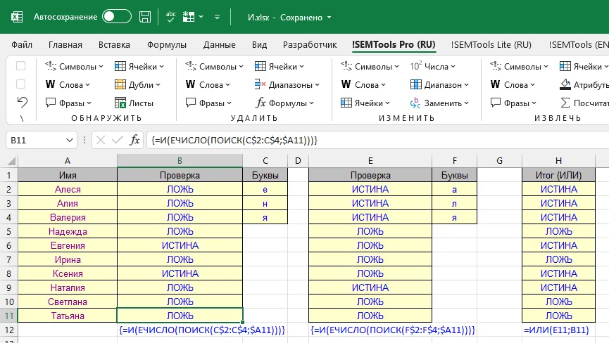
In column H, the OR function was useful - it passes names if they contain TRUE for at least one of the letter sets.
Other Logical functions in Excel
IF, OR, NOT, TRUE, FALSE, IFERROR, IFS, SWITCH, XOR
Like the article? Help its author! Buy !SEMTools, it has lots of useful instruments to process text data.