| Function category | Math |
| Volatility | Non-volatile |
| Similar functions | COUNTIFS, SUMIF, SUMPRODUCT |
The SUMIFS function is one of the most useful and powerful Excel functions for data analysis. It allows you to sum values from a specific range that meet multiple criteria simultaneously. If you work with large volumes of data and need to perform complex calculations with conditions, this function will become your indispensable assistant.
What is the SUMIFS function?
SUMIFS is a function that sums cells in a range that meet several specified conditions. Unlike SUMIF, which works with only one criterion, SUMIFS can check up to 127 different conditions in different ranges.
SUMIFS function syntax
=SUMIFS(sum_range, criteria_range1, criteria1, criteria_range2, criteria2, ...)- sum_range — range of cells to sum
- criteria_range1 — first range to which the condition applies
- criteria1 — first condition in the form of a number, expression, or text
- criteria_range2, criteria2, ... — additional pairs of ranges and conditions
| A | B | C | D | E | F | G | H | |
|---|---|---|---|---|---|---|---|---|
| 1 | Region | Product | Manager | Month | Sales | Condition | Result | |
| 2 | North | Table | Smith | January | 62000 | North | 139000=SUMIFS(E2:E8,A2:A8,"North") | |
| 3 | South | Table | Brown | January | 18000 | North + Table | 103000=SUMIFS(E2:E8,A2:A8,"North",B2:B8,"Table") | |
| 4 | North | Chair | Smith | February | 9000 | North + Table + January | 62000=SUMIFS(E2:E8,A2:A8,"North",B2:B8,"Table",D2:D8,"January") | |
| 5 | North | Table | Brown | February | 41000 | |||
| 6 | Center | Armchair | Smith | January | 75000 | |||
| 7 | South | Kommode | Jones | February | 33000 | |||
| 8 | North | Computer table | Jones | January | 27000 |
Each new “range, criterion” pair narrows the selection: a row is summed only if it meets all conditions. “Computer table” isn’t counted as “Table” — a criterion without wildcards requires an exact match.
SUMIFS features and limitations
Here are important rules and features of formulas with the SUMIFS function.
Range sizes
All ranges in the SUMIFS function must be the same size. If the sum range has 10 rows, then all criteria ranges must also contain 10 rows.
| A | B | C | D | E | |
|---|---|---|---|---|---|
| 1 | Region | Sales | Formula | Result | |
| 2 | North | 100 | same size | 300=SUMIFS(B2:B4,A2:A4,"North") | |
| 3 | South | 50 | different size | #VALUE!=SUMIFS(B2:B4,A2:A3,"North") | |
| 4 | North | 200 |
Unlike SUMIF, which silently adjusts the ranges, SUMIFS returns #VALUE! when the sizes don’t match.
Text criteria
Text criteria must be enclosed in double quotes. If you reference a cell with a criterion, quotes are not needed.
=SUMIFS(B2:B100, A2:A100, D1)| A | B | C | D | E | F | G | H | |
|---|---|---|---|---|---|---|---|---|
| 1 | Region | Sales | Region? | Result | Threshold | Above threshold | ||
| 2 | North | 100 | North | 300=SUMIFS(B2:B5,A2:A5,D2) | 90 | 450=SUMIFS(B2:B5,B2:B5,">"&G2) | ||
| 3 | South | 50 | ||||||
| 4 | North | 200 | ||||||
| 5 | south | 150 |
A cell reference is written without quotes. If it needs an operator, the operator goes in quotes and the cell is joined with an ampersand: ">"&G2. Case doesn’t matter: “south” and “South” are the same.
Case sensitivity
The SUMIFS function is not case-sensitive. Conditions "PRODUCT", "product", and "Product" will be treated the same.
SUMIFS usage examples
Download the file with all examples using this link.
Example 1: Sales sum by region and product
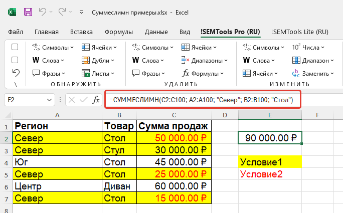
Suppose we have a sales table and we want to know the sum of sales for the product "Table" in the "North" region.
=SUMIFS(C2:C100, A2:A100, "North", B2:B100, "Table")| A | B | C | D | E | F | G | H | |
|---|---|---|---|---|---|---|---|---|
| 1 | Region | Product | Manager | Month | Sales | Condition | Result | |
| 2 | North | Table | Smith | January | 62000 | North and Table | 103000=SUMIFS(E2:E8,A2:A8,"North",B2:B8,"Table") | |
| 3 | South | Table | Brown | January | 18000 | |||
| 4 | North | Chair | Smith | February | 9000 | |||
| 5 | North | Table | Brown | February | 41000 | |||
| 6 | Center | Armchair | Smith | January | 75000 | |||
| 7 | South | Kommode | Jones | February | 33000 | |||
| 8 | North | Computer table | Jones | January | 27000 |
Rows 2 and 5 are summed: region “North” and product exactly “Table”.
Example 2: Sales sum above specific value
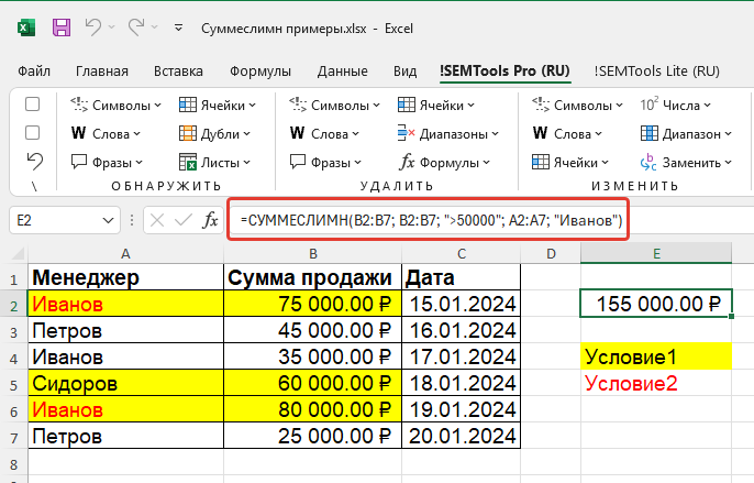
Let's say we need to calculate the sum of all sales that are greater than $50,000 and were made by manager “Smith”.
=SUMIFS(D2:D100, D2:D100, ">50000", E2:E100, "Smith")| A | B | C | D | E | F | G | H | |
|---|---|---|---|---|---|---|---|---|
| 1 | Region | Product | Manager | Month | Sales | Condition | Result | |
| 2 | North | Table | Smith | January | 62000 | > 50000 and Smith | 137000=SUMIFS(E2:E8,E2:E8,">50000",C2:C8,"Smith") | |
| 3 | South | Table | Brown | January | 18000 | |||
| 4 | North | Chair | Smith | February | 9000 | |||
| 5 | North | Table | Brown | February | 41000 | |||
| 6 | Center | Armchair | Smith | January | 75000 | |||
| 7 | South | Kommode | Jones | February | 33000 | |||
| 8 | North | Computer table | Jones | January | 27000 |
The sum range can also be a criteria range — that’s how you pick large deals.
SUMIFS with comparison operators
You can use various comparison operators in SUMIFS criteria:
Example 3: Sales sum in specific range
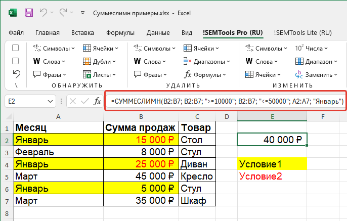
Let's find the sum of sales from $10,000 to $50,000 for January.
=SUMIFS(B2:B100, B2:B100, ">=10000", B2:B100, "<=50000", C2:C100, "January")| A | B | C | D | E | F | G | H | |
|---|---|---|---|---|---|---|---|---|
| 1 | Region | Product | Manager | Month | Sales | Condition | Result | |
| 2 | North | Table | Smith | January | 62000 | 10000–50000, January | 45000=SUMIFS(E2:E8,E2:E8,">=10000",E2:E8,"<=50000",D2:D8,"January") | |
| 3 | South | Table | Brown | January | 18000 | 10000–50000, total | 119000=SUMIFS(E2:E8,E2:E8,">=10000",E2:E8,"<=50000") | |
| 4 | North | Chair | Smith | February | 9000 | |||
| 5 | North | Table | Brown | February | 41000 | |||
| 6 | Center | Armchair | Smith | January | 75000 | |||
| 7 | South | Kommode | Jones | February | 33000 | |||
| 8 | North | Computer table | Jones | January | 27000 |
An interval is two conditions on the same range: the lower and the upper bound. The formula in the article filters by January, so the text now says January instead of the first quarter.
Example 4: Sales sum excluding specific product
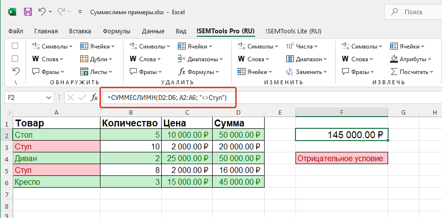
Let's calculate the sum of all sales except the product "Chair".
=SUMIFS(D2:D100, B2:B100, "<>Chair")| A | B | C | D | E | F | G | H | |
|---|---|---|---|---|---|---|---|---|
| 1 | Region | Product | Manager | Month | Sales | Condition | Result | |
| 2 | North | Table | Smith | January | 62000 | not Chair | 256000=SUMIFS(E2:E8,B2:B8,"<>Chair") | |
| 3 | South | Table | Brown | January | 18000 | not Chair, not Table | 135000=SUMIFS(E2:E8,B2:B8,"<>Chair",B2:B8,"<>Table") | |
| 4 | North | Chair | Smith | February | 9000 | |||
| 5 | North | Table | Brown | February | 41000 | |||
| 6 | Center | Armchair | Smith | January | 75000 | |||
| 7 | South | Kommode | Jones | February | 33000 | |||
| 8 | North | Computer table | Jones | January | 27000 |
“<>” means “not equal”. Several exclusions are several pairs with the same range.
SUMIFS with wildcards
You can use wildcards in SUMIFS criteria:
- * — any number of any characters
- ? — one any character
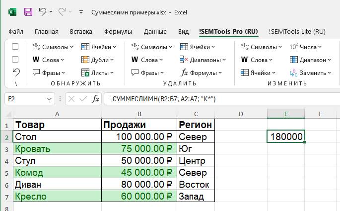
Example 5: Sales sum of products starting with specific letter
Let's find the sum of sales of all products whose name starts with "K".
=SUMIFS(C2:C100, A2:A100, "K*")| A | B | C | D | E | F | G | H | |
|---|---|---|---|---|---|---|---|---|
| 1 | Region | Product | Manager | Month | Sales | Condition | Result | |
| 2 | North | Table | Smith | January | 62000 | "K*" | 33000=SUMIFS(E2:E8,B2:B8,"K*") | |
| 3 | South | Table | Brown | January | 18000 | |||
| 4 | North | Chair | Smith | February | 9000 | |||
| 5 | North | Table | Brown | February | 41000 | |||
| 6 | Center | Armchair | Smith | January | 75000 | |||
| 7 | South | Kommode | Jones | February | 33000 | |||
| 8 | North | Computer table | Jones | January | 27000 |
The asterisk stands for any number of characters, so “Kommode” matches. In the article’s formula the products are in column A — use your own column.
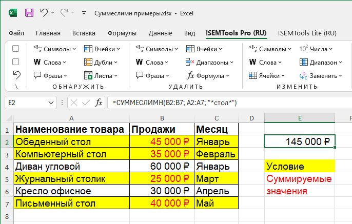
Example 6: Sales sum of products with specific pattern in name
Let's find the sum of sales of products that have "table" anywhere in their name.
=SUMIFS(D2:D100, B2:B100, "*table*")| A | B | C | D | E | F | G | H | |
|---|---|---|---|---|---|---|---|---|
| 1 | Region | Product | Manager | Month | Sales | Condition | Result | |
| 2 | North | Table | Smith | January | 62000 | "*table*" | 148000=SUMIFS(E2:E8,B2:B8,"*table*") | |
| 3 | South | Table | Brown | January | 18000 | "Table" exactly | 121000=SUMIFS(E2:E8,B2:B8,"Table") | |
| 4 | North | Chair | Smith | February | 9000 | |||
| 5 | North | Table | Brown | February | 41000 | |||
| 6 | Center | Armchair | Smith | January | 75000 | |||
| 7 | South | Kommode | Jones | February | 33000 | |||
| 8 | North | Computer table | Jones | January | 27000 |
With asterisks on both sides “Computer table” is included too. Without them — only an exact match.
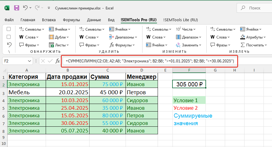
Example 7: Sales analysis by dates and categories
Suppose we need to calculate the sum of sales for the "Electronics" category for the first half of 2024.
=SUMIFS(E2:E1000, C2:C1000, "Electronics", D2:D1000, ">=01/01/2024", D2:D1000, "<=06/30/2024")| A | B | C | D | E | F | G | |
|---|---|---|---|---|---|---|---|
| 1 | Category | Date | Sales | From | To | Result | |
| 2 | Electronics | 01/05/2024 | 12000 | 01/01/2024 | 06/30/2024 | 42000=SUMIFS(C2:C6,A2:A6,"Electronics",B2:B6,">="&E2,B2:B6,"<="&F2) | |
| 3 | Furniture | 02/14/2024 | 30000 | 42000=SUMIFS(C2:C6,A2:A6,"Electronics",B2:B6,">="&DATE(2024,1,1),B2:B6,"<="&DATE(2024,6,30)) | |||
| 4 | Electronics | 06/30/2024 | 8000 | ||||
| 5 | Electronics | 07/01/2024 | 15000 | ||||
| 6 | Electronics | 03/20/2024 | 22000 |
06/30/2024 is included (“<=”), 07/01/2024 is not. Keep the boundary dates in cells (E2, F2) or build them with DATE(): a date typed inside quotes like ">=01/01/2024" depends on the regional settings.
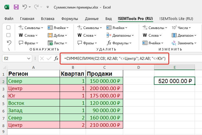
Example 8: Summing with multiple exclusions
Let's calculate the sum of sales for all regions except "Center" and "South".
=SUMIFS(F2:F500, A2:A500, "<>Center", A2:A500, "<>South")| A | B | C | D | E | F | G | H | |
|---|---|---|---|---|---|---|---|---|
| 1 | Region | Product | Manager | Month | Sales | Condition | Result | |
| 2 | North | Table | Smith | January | 62000 | not Center, not South | 139000=SUMIFS(E2:E8,A2:A8,"<>Center",A2:A8,"<>South") | |
| 3 | South | Table | Brown | January | 18000 | |||
| 4 | North | Chair | Smith | February | 9000 | |||
| 5 | North | Table | Brown | February | 41000 | |||
| 6 | Center | Armchair | Smith | January | 75000 | |||
| 7 | South | Kommode | Jones | February | 33000 | |||
| 8 | North | Computer table | Jones | January | 27000 |
Only “North” remains. Exclusions combine with AND: a row must differ from every listed value.
SUMIFS with OR logic
All SUMIFS conditions work as AND. To sum “North OR South”, pass the values as an array constant and wrap the formula in SUM — SUMIFS calculates a total for each value, and SUM adds them up.
| A | B | C | D | E | F | G | H | |
|---|---|---|---|---|---|---|---|---|
| 1 | Region | Product | Manager | Month | Sales | Condition | Result | |
| 2 | North | Table | Smith | January | 62000 | North or South | 190000=SUM(SUMIFS(E2:E8,A2:A8,{"North","South"})) | |
| 3 | South | Table | Brown | January | 18000 | (North or South) and Table | 121000=SUM(SUMIFS(E2:E8,A2:A8,{"North","South"},B2:B8,"Table")) | |
| 4 | North | Chair | Smith | February | 9000 | |||
| 5 | North | Table | Brown | February | 41000 | |||
| 6 | Center | Armchair | Smith | January | 75000 | |||
| 7 | South | Kommode | Jones | February | 33000 | |||
| 8 | North | Computer table | Jones | January | 27000 |
Curly braces define an array constant. Don’t use arrays in two different criteria at once — Excel pairs the elements instead of combining every option.
SUMIFS vs SUMIF
SUMIF takes one condition, and its sum range comes last; in SUMIFS it comes first. That’s why SUMIFS is convenient even for one condition: you can add more without reordering the arguments.
| A | B | C | D | E | F | G | H | |
|---|---|---|---|---|---|---|---|---|
| 1 | Region | Product | Manager | Month | Sales | Condition | Result | |
| 2 | North | Table | Smith | January | 62000 | SUMIF | 139000=SUMIF(A2:A8,"North",E2:E8) | |
| 3 | South | Table | Brown | January | 18000 | SUMIFS | 139000=SUMIFS(E2:E8,A2:A8,"North") | |
| 4 | North | Chair | Smith | February | 9000 | |||
| 5 | North | Table | Brown | February | 41000 | |||
| 6 | Center | Armchair | Smith | January | 75000 | |||
| 7 | South | Kommode | Jones | February | 33000 | |||
| 8 | North | Computer table | Jones | January | 27000 |
Same result — only the order of the arguments differs.
Summary: when to use SUMIFS
The SUMIFS function is a powerful tool for multi-factor data analysis in Excel. By mastering it, you can efficiently sum data based on multiple conditions and get accurate results for making informed business decisions.
Like the article? Help its author! Buy !SEMTools, it has lots of useful instruments to process text data.