FIND Function in Excel: Case-Sensitive Text Search

FIND function examples in Excel — FIND function usage examples

Function category	Text
Volatility	Non-volatile
Similar functions	SEARCH, Find and Replace (procedure)

What does the FIND function do?

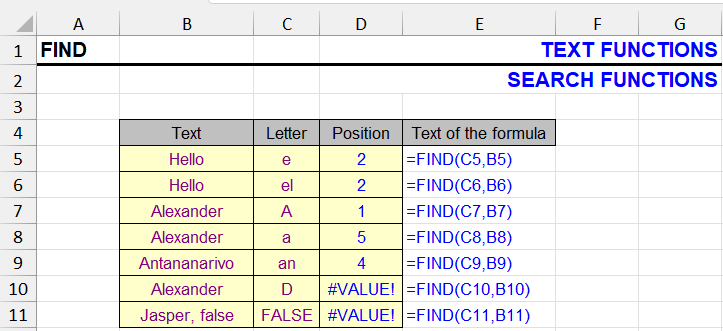
This function searches for text within another text fragment using case-sensitive search. This distinguishes it from the SEARCH function, despite having an absolutely identical syntax. The second difference - it doesn't support wildcard characters, treating them as regular characters.

When the search text is found, its position in the text is displayed as a number. If the text contains more than one occurrence, the position of the first one is output.

The third optional parameter is used to find a fragment starting from a specific position in the text.

If the search text is not found in the text, the function returns a #VALUE! error.

FIND - Function syntax

Syntax of the "FIND" function:

=FIND(Find_Text, Within_Text, Start_Position)

FIND is case-sensitive, SEARCH isn’t Formulas

D3=FIND(A3,B3,C3)

	A	B	C	D	E
1	Find_Text	Within_Text	Start	FIND	SEARCH
2	a	Banana	1	2=FIND(A2,B2,C2)	2=SEARCH(A2,B2,C2)
3	A	Banana	1	#VALUE!=FIND(A3,B3,C3)	2=SEARCH(A3,B3,C3)
4	B	Banana	1	1=FIND(A4,B4,C4)	1=SEARCH(A4,B4,C4)
5	a	Banana	3	4=FIND(A5,B5,C5)	4=SEARCH(A5,B5,C5)
6	-	A-12-B	3	5=FIND(A6,B6,C6)	5=SEARCH(A6,B6,C6)
7	x	Banana	1	#VALUE!=FIND(A7,B7,C7)	#VALUE!=SEARCH(A7,B7,C7)

FIND finds no “A” in “Banana” (#VALUE!), SEARCH finds “a” at 2. Start_Position 3 skips the first two characters: the next “a” is at 4, the next “-” at 5.

FIND: result and input format

See SEARCH function

FIND function - examples

If case is not important, it's better to use the SEARCH function and take examples from there.

Find uppercase letters with an array constant

The function is case-sensitive, which allows using it, for example, to find uppercase letters in Excel. The solution below, however, is not the most elegant, there are simpler options (in the article via the link).

=COUNT(FIND({"A","B","C","D","E","F","G","H","I","J","K","L","M","N","O","P","Q","R","S","T","U","V","W","X","Y","Z"}, A1)) > 0

Uppercase letters with an array constant Formulas

B3=COUNT(FIND({"A","B","C","D","E","F","G","H","I","J","K","L","M","N","O","P","Q","R","S","T","U","V","W","X","Y","Z"},A3))>0

	A	B
1	Text	Has an uppercase letter?
2	report final	FALSE=COUNT(FIND({"A","B","C","D","E","F","G","H","I","J","K","L","M","N","O","P","Q","R","S","T","U","V","W","X","Y","Z"},A2))>0
3	Report final	TRUE=COUNT(FIND({"A","B","C","D","E","F","G","H","I","J","K","L","M","N","O","P","Q","R","S","T","U","V","W","X","Y","Z"},A3))>0
4	iPhone	TRUE=COUNT(FIND({"A","B","C","D","E","F","G","H","I","J","K","L","M","N","O","P","Q","R","S","T","U","V","W","X","Y","Z"},A4))>0
5	no caps here 123	FALSE=COUNT(FIND({"A","B","C","D","E","F","G","H","I","J","K","L","M","N","O","P","Q","R","S","T","U","V","W","X","Y","Z"},A5))>0

FIND looks for all 26 letters at once and returns 26 results: positions or #VALUE!. COUNT counts only the numbers, so > 0 means at least one uppercase letter was found.

Find uppercase English letters in a cell

The formula above lists all 26 letters manually. A more elegant way is an array formula that generates them itself.

The COUNT function and CHAR function will help compose such a formula:

{=COUNT(FIND(CHAR(ROW(65:90)), A1)) > 0}

Uppercase letters with CHAR(ROW(65:90)) Formulas

B2=COUNT(FIND(CHAR(ROW($65:$90)),A2))>0

	A	B	C	D
1	Text	Uppercase?	How many uppercase letters	Position of the first
2	New York	TRUE=COUNT(FIND(CHAR(ROW($65:$90)),A2))>0	2=COUNT(FIND(CHAR(ROW($65:$90)),A2))	1=MIN(IFERROR(FIND(CHAR(ROW($65:$90)),A2),""))
3	iPhone 15 Pro	TRUE=COUNT(FIND(CHAR(ROW($65:$90)),A3))>0	1=COUNT(FIND(CHAR(ROW($65:$90)),A3))	2=MIN(IFERROR(FIND(CHAR(ROW($65:$90)),A3),""))
4	lowercase	FALSE=COUNT(FIND(CHAR(ROW($65:$90)),A4))>0	0=COUNT(FIND(CHAR(ROW($65:$90)),A4))	0=MIN(IFERROR(FIND(CHAR(ROW($65:$90)),A4),""))
5	ABBA	TRUE=COUNT(FIND(CHAR(ROW($65:$90)),A5))>0	2=COUNT(FIND(CHAR(ROW($65:$90)),A5))	1=MIN(IFERROR(FIND(CHAR(ROW($65:$90)),A5),""))

CHAR(ROW(65:90)) builds the letters A–Z. COUNT without “> 0” shows how many different uppercase letters the text has: “ABBA” has 2 (A and B). MIN of the positions gives the first one; 0 means none. In Excel 365 no Ctrl+Shift+Enter is needed.

The formula will also return TRUE or FALSE.

Important: the array formula is entered without curly braces using the Ctrl + Shift + Enter key combination.