
| Function category | Text |
| Volatility | Non-volatile |
What does the REPT function do?
This function repeats a text fragment a specified number of times.
You need to specify the text to repeat and how many times to repeat it.
In the latest versions of Excel, the function will return a #VALUE! error if the returned value exceeds 32767 characters.
REPT function syntax
=REPT(Text, Number_times)| A | B | C | |
|---|---|---|---|
| 1 | Text | Number_times | REPT |
| 2 | ab | 3 | ababab=REPT(A2,B2) |
| 3 | * | 5 | *****=REPT(A3,B3) |
| 4 | - | 2.9 | --=REPT(A4,B4) |
| 5 | x | 0 | =REPT(A5,B5) |
| 6 | x | -1 | #VALUE!=REPT(A6,B6) |
| 7 | =REPT("0",5-LEN(A8))&A8 | 00042=REPT("0",5-LEN(42))&42 |
A fractional count is truncated (2.9 → 2), 0 gives an empty string, a negative number gives #VALUE!. The last row pads a number with leading zeros to 5 characters.
REPT formula examples
Example 1
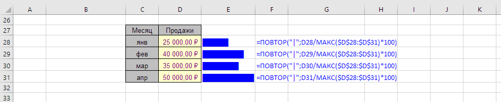
The table above was used to create a simple histogram of sales indicators.
The REPT function uses the sales value divided by the maximum value from the same table so that the number of repetitions doesn't exceed 100.
To prevent spaces from displaying between the "l" symbols, the Playbill font was used.
| A | B | C | |
|---|---|---|---|
| 1 | Region | Sales | Bar |
| 2 | North | 8200 | ██████████████=REPT("█",B2/MAX($B$2:$B$5)*20) |
| 3 | South | 5400 | █████████=REPT("█",B3/MAX($B$2:$B$5)*20) |
| 4 | East | 12000 | ████████████████████=REPT("█",B4/MAX($B$2:$B$5)*20) |
| 5 | West | 2600 | ████=REPT("█",B5/MAX($B$2:$B$5)*20) |
Each bar is up to 20 characters long: the value divided by the maximum, times 20 (REPT drops the fraction). The full block character █ (UNICHAR(9608)) draws a solid bar in any font, so you don’t need Playbill. Data bars in Conditional Formatting do the same without formulas.
This example is most useful for compatibility with Excel versions before 2010, since they didn't yet have the "Sparklines" tool.
Example 2
The REPT function is used in a complex formula to extract words containing a specific character.
The function is used to create a sufficiently large number of spaces between words (99 in this case).
Using the REPT function makes the formula more compact.
| A | B | |
|---|---|---|
| 1 | Text | First word with “#” |
| 2 | buy apples #sale today | #sale=TRIM(MID(SUBSTITUTE(A2," ",REPT(" ",99)),MAX(1,FIND("#",SUBSTITUTE(A2," ",REPT(" ",99)))-50),99)) |
| 3 | new #promo and #sale | #promo=TRIM(MID(SUBSTITUTE(A3," ",REPT(" ",99)),MAX(1,FIND("#",SUBSTITUTE(A3," ",REPT(" ",99)))-50),99)) |
| 4 | no tags here | #VALUE!=TRIM(MID(SUBSTITUTE(A4," ",REPT(" ",99)),MAX(1,FIND("#",SUBSTITUTE(A4," ",REPT(" ",99)))-50),99)) |
REPT(" ",99) turns every space into 99 spaces, so a 99-character window around the “#” contains only one word; TRIM removes the padding. No “#” → #VALUE!.
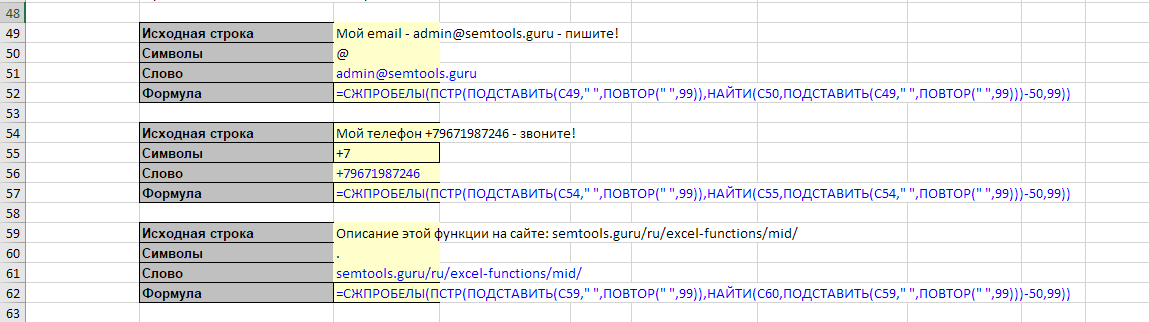
See examples of such usage in the articles:
Like the article? Help its author! Buy !SEMTools, it has lots of useful instruments to process text data.