LEFT

What does LEFT do?

Returns the first N characters of text from the left.

LEFT syntax

=LEFT(Text, Number_Characters)

The second argument, the number of characters to extract, is optional and by default (if not specified) equals 1, meaning the formula result will be the first character.

If the second argument equals or exceeds the string length, the entire original cell text is returned.

If it equals zero – an empty string is returned.

If a negative number is specified, a #VALUE! error is returned.

LEFT – formatting

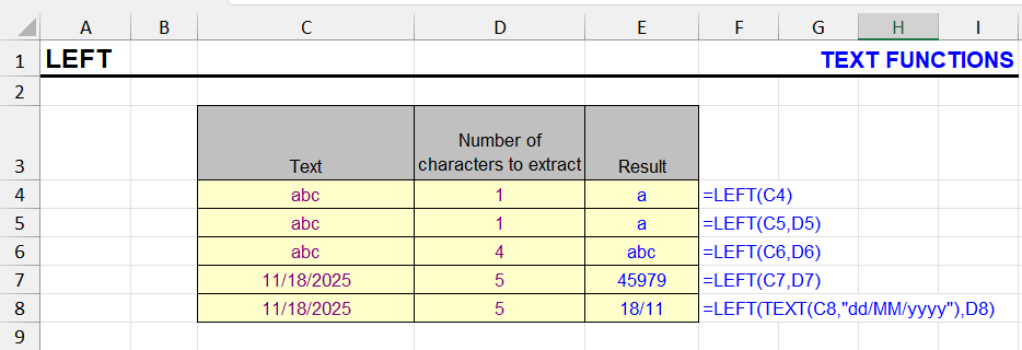
It’s important to note that if the first argument is a cell with a date or date-time, or a formula returning them, the LEFT function will convert them to a natural number and only then to a string value.

Therefore, for correct text extraction of part of characters from dates in numeric format, the TEXT function may be needed (see example in the image above).

Formula examples with the LEFT function

Let’s consider examples of using the LEFT function in practice.

Example 1 – extract first word

In this simplest example, we extract the first word in a cell using a combination of LEFT and FIND functions.

=LEFT(A1, FIND(" ", A1) - 1)

The table above was used to extract the first name from a string containing first and last name. The FIND function is used to determine the position of the space between first and last name. Therefore, the length of the first name is the space position minus one character.
The LEFT function extracts the first name based on its length.

How to extract the last name (second word)? See the answer in the description of the RIGHT function.

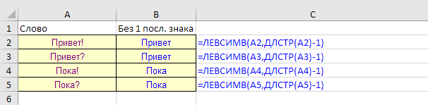
Example 2 – extract everything except last character

In combination of LEFT with the LEN function, we extract from strings of variable length everything except the last character.

Example 3 – extract text before first digit (array formula)

In the lighting catalog, the collection name is always represented by a text designation. The article number of a specific product always starts with digits. The task is to extract from the product name its collection without the article number.

So, the task is to extract characters before any first digit. Let’s do this using a combination of LEFT with MIN and SEARCH functions.

The formula borrows mechanics from the first example but is an array formula and looks as follows:

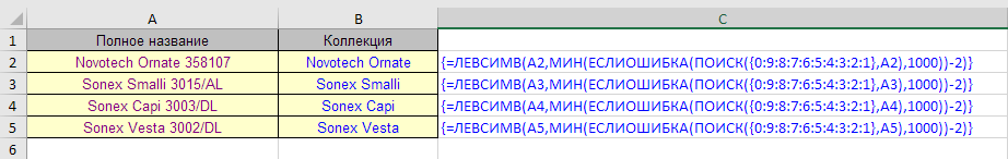
This is what the formula for cell A1 will look like.

=LEFT(A1, MIN(IFERROR(SEARCH({0,9,8,7,6,5,4,3,2,1}, A1), 1000)) - 2)

The formula is entered with the Ctrl + Shift + Enter key combination, like any array formula. But if you have Office 365 or Excel 2021 (and later) – then you can just use the Enter key.

How the formula works:

1. The SEARCH function simultaneously searches for 10 digits listed in the array and returns an array of positions
2. Since some digits return errors when searched, the IFERROR function is used to return a deliberately large number (in this case 1000) for such values
3. The MIN function returns the smallest of the numbers – this will be the position of the first digit in the string
4. Since there’s always a space before the digits, 2 characters are subtracted, not 1. You can be safe in case of missing spaces – leave 1 and remove spaces with the TRIM function
5. The LEFT function returns text up to the calculated position of the last character that comes before the first digit and the space before it

This post is also available in RU.