| Function category | Text |
| Volatility | Non-volatile |
| Similar functions | FIND, find and replace (procedure) |
What does the SEARCH function do?
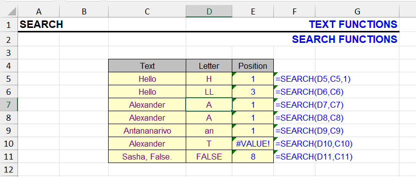
This function is similar to the FIND function and also searches for a substring within a string. When the search text is found, its position in the text is displayed as a number.
The difference from the FIND function is that SEARCH is case-insensitive. Both for the search text and the text being searched. It also supports wildcard operators.
Both functions have a procedure-analog Find and Replace – as a procedure, it has its own advantages and disadvantages.
Syntax
=SEARCH(Find_Text, Within_Text, [Start_Position])- Find_Text — character or combination being searched for
- Within_Text — cell, text value, or any expression returned by another function
- Start_Position — optional parameter, if omitted search starts from the first character
If the text contains more than one occurrence, the position of the first one is returned.
The third (optional) parameter is used to search from a specific position in the text and defaults to 1.
If the search text is not found in the text, the function returns a #VALUE! error.
Formatting
When searching for dates, the SEARCH function, like all text functions, treats them as numbers, so for correct searching the TEXT function may be needed.
Meanwhile, logical values TRUE and FALSE are converted to text corresponding to their spelling.
Search for a character in a cell
The simplest example of using the function is searching for a specific character in a cell.
The logic is simple – if searching for the character’s position doesn’t return an error, then the character is present in the cell:
=NOT(ISERROR(SEARCH(pattern, text)))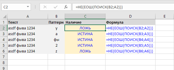
Extract first word
In this simplest example, we extract the first word from a cell using the combination — LEFT function + SEARCH function. Since space is a case-insensitive character, for this case you could also use the FIND function.
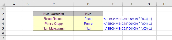
The table above was used to extract the first name from a string containing first and last name.
- SEARCH returns the position of the space between first and last name
- The length of the first name is calculated as the space position minus 1
- LEFT function extracts the first name based on its length
Other usage examples
Find the first digit in a cell:
=MIN(IFERROR(SEARCH({0,9,8,7,6,5,4,3,2,1}, A1), 1000))Find the first digit in a cell and return everything before it:
=LEFT(A1, MIN(IFERROR(SEARCH({0,9,8,7,6,5,4,3,2,1}, A1), 1000)) - 1)Check if a cell contains Latin characters. The formula returns “TRUE” or “FALSE”:
=COUNT(SEARCH({"a","b","c","d","e","f","g","h","i","j","k","l","m","n","o","p","q","r","s","t","u","v","w","x","y","z"}, A1)) > 0SEARCH function in array formula
The examples above, where letters are explicitly listed in a string array, take up quite a lot of space. The letters go in sequence, which suggests they could be expressed as a range differently.
And indeed, this is possible using a combination with ROW and SEARCH functions:
{=COUNT(SEARCH(CHAR(ROW(65:90)), A1)) > 0}The difference between this array formula and the previous ones is that it needs to be entered without curly braces, they will appear when entering the formula with Ctrl + Shift + Enter (instead of regular Enter). In the formula above where all letters are explicitly listed, curly braces are entered manually – this is an explicit indication of a string array.
What happens in this formula?
- The ROW function with numerical argument “65:90” returns an array of numbers from 65 to 90 inclusive. Exactly in this range in the ASCII table are all Latin characters;
- CHAR function returns for each numerical value in this array its character, thus creating an array of Latin characters;
- The SEARCH function searches for each of these characters in the string and returns either a number or an error, thus creating an array of numbers and errors
- The COUNT function counts numerical values in the resulting array. If the result is greater than zero, then at least one Latin character was found. If not (all searches returned an error), then none were found
Similar formula for Cyrillic:
{=COUNT(SEARCH(CHAR(ROW(192:223)), A1)) > 0}Read more about finding and extracting Cyrillic and Latin characters in Excel here:
There are many more combinations of the SEARCH function with other Excel functions, see sections:
OR function
AND function
VALUE function
Remove first word in Excel cell
See also on this topic:
Finding tools (!SEMTools add-in functionality)
Regular expressions in Excel
Find specific characters in Excel
Like the article? Help its author! Buy !SEMTools, it has lots of useful instruments to process text data.