| Function category | Math |
| Volatility | Non-volatile |
| Similar functions | ROW, COLUMN, INDIRECT |
The SEQUENCE function is available in modern versions of Excel, including Excel for Microsoft 365, Excel 2021 and Excel 2024. It is part of the dynamic array functions family that fundamentally changed the approach to working with data arrays in Excel. Dynamic arrays automatically expand and shrink, adjusting to the volume of returned data, which eliminates the need for manual management of output range sizes.
What does the SEQUENCE function do
The SEQUENCE function is designed to generate number sequences as dynamic arrays. Its main task is to return an ordered set of numbers that automatically fills the specified cell range. Unlike static methods of creating sequences, the function’s result dynamically updates when source parameters or table data change.
In previous versions of Excel, the ROW, COLUMN and INDIRECT functions were used in array formulas to output number sequences.
Syntax, arguments of the SEQUENCE function
The SEQUENCE function syntax is quite complex. It has 4 numeric arguments:
=SEQUENCE(rows, [columns], [start], [step])Only the first argument (rows) is mandatory, the other arguments can be omitted, their value is already set by default as 1 (the most common case).
When entering the function using the Shift + F3 key combination through the function insert window, you can view the list of arguments and enter them in the appropriate fields:
Let me explain the arguments in more detail.
Required argument: rows
The first argument (rows) determines the number of rows that the resulting sequence will occupy. This is the only required argument of the function. For example, the formula =SEQUENCE(5) returns an array of numbers from 1 to 5, located in five consecutive cells of one column.
Optional argument: columns
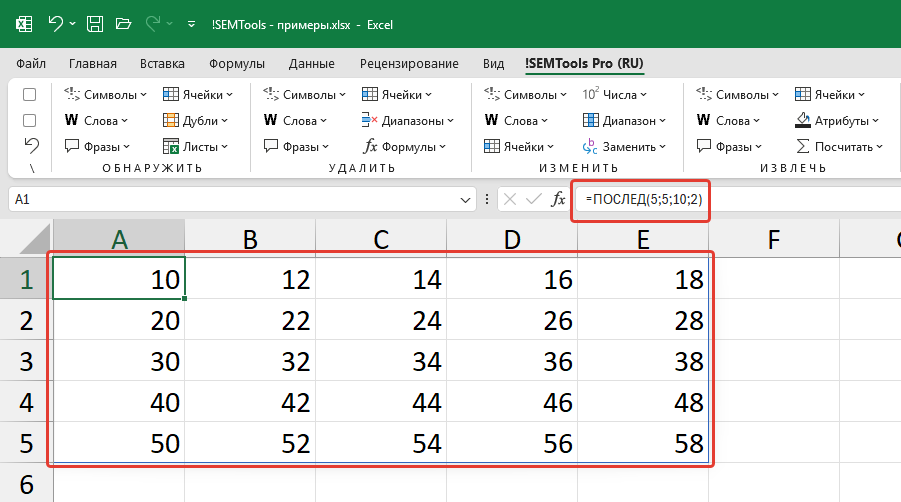
The columns argument sets the number of columns for the output array. If the argument is not specified, the default value is 1. When both arguments are specified, a two-dimensional array is created. For example, =SEQUENCE(3,3) creates a 3×3 matrix, filling it with numbers from 1 to 9. By default, filling occurs from left to right, then top to bottom.
Optional argument: start
The start argument determines the first number in the sequence. If the argument is omitted, the sequence starts with 1. The argument supports negative and fractional values. For example, =SEQUENCE(3,1,5) will return the array [5; 6; 7].
Optional argument: step
The step argument sets the difference between adjacent elements of the sequence. By default, step 1 is used. Like the starting value, step can be negative (for decreasing sequences) or fractional. For example,
=SEQUENCE(4,1,0,2.5)
will create the sequence [0; 2.5; 5; 7.5].
Filling direction and the TRANSPOSE function
By default, the SEQUENCE function fills the array by rows. To change the filling direction, the TRANSPOSE function is used, which changes the orientation of the array. For example,
=TRANSPOSE(SEQUENCE(3, 3))transforms a horizontal sequence into a vertical one, effectively swapping rows and columns in the resulting array.
Advantages of the SEQUENCE function
The function offers several advantages compared to traditional techniques, data organization methods and functions. Let’s look at a few examples.
SEQUENCE vs Static constant arrays
Static arrays, written in the {1;2;3;4;5} format, are immutable constants. Their size and values are fixed at creation time and cannot be recalculated based on other cells or formulas. Changing such an array requires its complete redefinition.
SEQUENCE creates calculated arrays whose parameters can depend on other cells in the table. For example, =SEQUENCE(A1) will automatically change size when the value in cell A1 changes. This allows creating adaptive data structures that are unavailable when using constant arrays.
SEQUENCE vs ROW/COLUMN function combinations
Traditionally, combinations of ROW and COLUMN functions were used to create sequences. For example, =ROW(A1) when dragged gives the sequence 1, 2, 3… For complex cases, formulas like =ROW(A1)-ROW(A$1) were required, which complicated reading and editing.
The SEQUENCE function provides a direct and intuitive solution for the same tasks. The formula =SEQUENCE(5) replaces dragging five cells with ROW formulas. For creating two-dimensional arrays, the difference is even more significant: one SEQUENCE formula replaces complex matrix constructions based on ROW/COLUMN.
The key advantage of SEQUENCE is the ability to create complete arrays “in one shot” without the need to fill a range with formulas. This is especially important when building complex dynamic reports and dashboards.
Examples of combinations with other functions
Outputting number sequences themselves to the sheet is not as interesting as using them together with other functions that have numeric arguments. And these are not necessarily mathematical or statistical functions. Text functions and date-time functions also often accept numeric arguments as input. Which means, number sequences too.
Examples of usage with text functions:
How to create alphabet in Excel
How to delete punctuation in Excel
How to find Latin characters in text.
Let’s consider other examples right in this article.
Dynamic numbered list with COUNTA
A numbering column is usually created by manually dragging values. But manual dragging creates static values that don’t adapt to changes in the table structure. When deleting a row in such a list, a numbering gap occurs (1, 2, 4, 5…), requiring manual correction. Adding new data also requires re-dragging the list.
The SEQUENCE function generates a dynamic array that automatically recalculates with any changes. In combination with the COUNTA function, you can build a numbering system that adapts to changes in the number of records:
=SEQUENCE(COUNTA(B:B), 1, 1, 1)Deleting or adding rows won’t break the sequence integrity, since the formula is recalculated each time, ensuring constant data correctness.
SEQUENCE combinations with FILTER, LARGE
With FILTER, the SEQUENCE function allows implementing sampling of every Nth element:
=FILTER(A:A, MOD(SEQUENCE(ROWS(A:A)), N) = 0)For data analysis, the combination with LARGE is useful. For example,
=LARGE(A:A, SEQUENCE(3))returns the three largest values from the range. This approach simplifies creating rankings and other ranked lists without changing the source data.
VLOOKUP + SEQUENCE for outputting multiple columns of values
The SEQUENCE function solves the classic limitation of VLOOKUP, allowing extraction of multiple columns simultaneously. The formula
=VLOOKUP(A2, $C$2:$F$100, SEQUENCE(1, 3, 2, 1), FALSE)returns three columns of data (from 2nd to 4th) for the lookup value. This eliminates the need to create separate formulas for each column and significantly simplifies the table structure.
Generating date sequences with the DATE function
The SEQUENCE function is effective for creating calendars and schedules. The formula
=DATE(2024, 1, SEQUENCE(31))generates all dates of January 2024. To learn how to avoid manually entering the number of days in a month, see this article: How to count the number of days in a month.
For workdays, the combination with WORKDAY.INTL is used:
=WORKDAY.INTL(START_DATE, SEQUENCE(30) - 1)creates a sequence of 30 workdays.
And in combination with the functions TODAY, YEAR, DATE and TEXT, you can create an ordered list of month names:
=TEXT(DATE(YEAR(TODAY()), SEQUENCE(12), 1), "MMMM")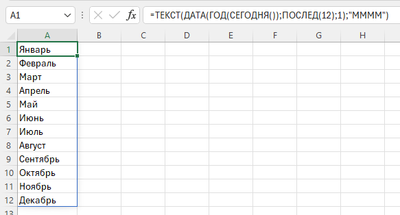
If you “wrap” the formula with the TRANSPOSE function, the list becomes horizontal. This eliminates the need to manually update report headers when the period changes.
Like the article? Help its author! Buy !SEMTools, it has lots of useful instruments to process text data.