| Function category | Math |
| Volatility | Non-volatile |
| Similar functions | SUM, SUMIF, PRODUCT |
| Similar procedures | Pivot tables |
What does this function do?
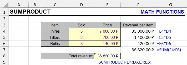
This function uses at least two ranges or arrays, multiplying and summing their elements.
Values in the first range are multiplied by corresponding values in the second range, and so on.
The sum of all such products is the calculation result.
Most often, the function is used as an alternative to the SUMIF function with multiple conditions.
- The advantage of SUMPRODUCT over pivot tables is that in pivot tables, the filter for creating a slice is always an exact match (as in example 1). And “filter by label,” if you output filtered values to rows, allows filtering by only one condition. SUMPRODUCT allows using all variants of string comparison (contains, starts with, ends with, matches) as well as numeric comparison (greater than, less than, equal to, not equal to, greater than or equal to, less than or equal to).
- The second advantage of SUMPRODUCT over pivot tables is that one filtering criterion in pivot tables cannot be used twice. SUMPRODUCT allows referencing the same column multiple times.
- The advantage of SUMPRODUCT over the SUMIFS function is that the conditional logic of SUMIFS is strictly “AND” for all conditions. The ability to use any logical operations on arrays of boolean values provides complete freedom to combine conditions in any logical combinations – AND, OR, IF, NOT.
Formatting
Ranges must be unidirectional, contain the same number of elements, and have the same vertical or horizontal dimensions. Specific range addresses don’t matter.
Ranges can have multiple columns and rows simultaneously. Typically, vertical ranges with a width of 1 column are used.
Function syntax
=SUMPRODUCT(range_or_array1, range_or_array2, …)Usage example
Let’s examine a complex example with 4 conditions in detail.
The marketer’s task is to calculate the sum based on four conditions:
- Week start date – April 13 or later
- Campaign name contains the word “Brand”
- Campaign ends with “BY” (Belarus)
- Or ends with “UA” (Ukraine)
Rows meeting all four conditions are highlighted in green. How to create a formula that would account for only them?
The formula can be seen in the screenshot in cell H9.
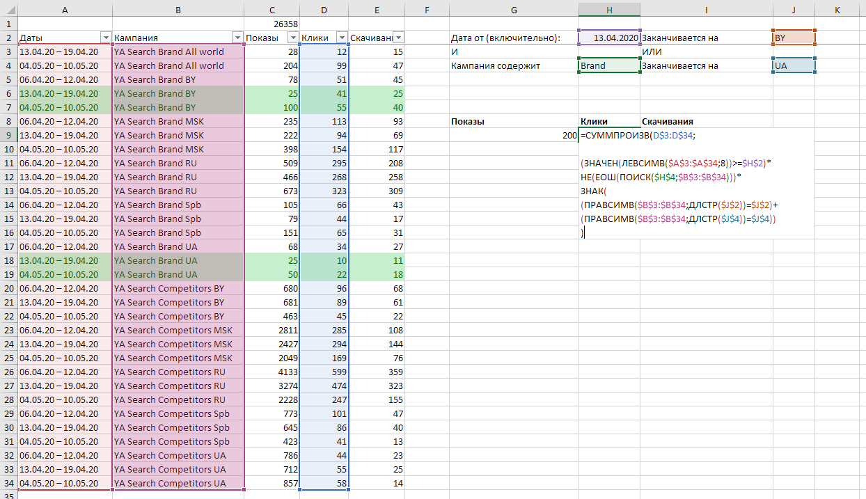
Essentially, it’s the sum of the product of two ranges – the array of numbers D3:D34 and an array of zeros and ones. Let’s examine it closer:
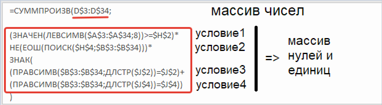
The array of zeros and ones is created by multiplying three array formulas, the third of which is obtained by adding two other array formulas and applying the SIGN function.
Each row shows one of the four conditions on which these formulas are based:
(VALUE(LEFT($A$3:$A$34, 8)) >= $H$2)This expression creates an array of boolean values TRUE and FALSE. The LEFT($A$3:$A$34,8) function extracts the first 8 characters from the date range in column A, and the VALUE function converts them to numeric format; otherwise, comparison with cell H2 won’t work correctly because the LEFT function is a text function and returns a string.
NOT(ISERROR(SEARCH($H$4, $B$3:$B$34)))This expression also creates an array of boolean values. The SEARCH function searches for the word “BRAND” inside each cell of column B; if not found, it returns an error, and if found, it returns the position of its first character in the string. With the ISERROR function we turn errors into ones and their absence into zeros. And then with the NOT function we get the array we need.
There’s no “Ends with” function in Excel, but you can do a simple check – if the last characters in the string match the word, isn’t that an occurrence? This operation is performed by the expression:
(RIGHT($B$3:$B$34, LEN($J$2)) = $J$2)Here we’re helped by the LEN and RIGHT functions. By checking whether the last 2 characters match cell J2, we also return an array of boolean values.
The fourth condition is similar to the third, as is its expression:
(RIGHT($B$3:$B$34, LEN($J$4)) = $J$4)The OR conditional logic is reproduced by adding two boolean arrays. In doing so, they become numbers. TRUE+FALSE (and vice versa) gives 1, FALSE+FALSE gives 0, TRUE+TRUE gives 2. To avoid distorting the data, we use the SIGN function – it returns 1 for positive numbers and 0 for 0. Thus, we get an array of zeros and ones based on two boolean arrays.
Multiplying the three arrays gives us a single array of zeros and ones. Multiplying this by the values of impressions, clicks, and downloads, we get the sums of values filtered this way. Numbers where conditions aren’t met are “destroyed” by zeros, and numbers where conditions are met are multiplied by 1 and summed.
An observant reader might wonder why we don’t use the OR function to combine the last two boolean arrays. The answer: unfortunately, it doesn’t combine arrays pairwise (just like the AND function), but considers each cell of the array as an equal element.
This is why arithmetic functions are used.
- Instead of AND – multiplication
- And instead of OR – addition + SIGN function.
Other examples with SUMPRODUCT:
Find duplicate values in Excel
Like the article? Help its author! Buy !SEMTools, it has lots of useful instruments to process text data.