| Function category | Lookup and reference functions |
| Volatility | Non-volatile |
| Similar functions | HLOOKUP, XLOOKUP |
The VLOOKUP function (Vertical Lookup) is quite simple to use. There are dozens of examples and even step-by-step tutorials available. However, Excel beginners often struggle to understand how formulas with VLOOKUP actually work.
In this article, I’ll try to explain in the simplest terms how VLOOKUP works and teach you how to use it effectively.
How VLOOKUP works – for beginners
The function name itself gives half the answer to “How does VLOOKUP work?” It stands for Vertical Lookup because it finds what you’re looking for by scanning data vertically in a table.
VLOOKUP function syntax
The VLOOKUP function syntax looks like this:
=VLOOKUP(lookup_value, table_array, col_index_num, range_lookup)
I’ve taught VLOOKUP syntax to many people and found that the most common difficulty is remembering the order of the function arguments – what comes after what.
When I think about this function, I remember the familiar TV show “What? Where? When?”
The first two arguments are exactly “What?” and “Where?” in that order. The first argument is the lookup value, in other words, what we’re looking for. The second argument is the range or table – simply put, where we’re looking. The third argument is a number that indicates when we should stop counting columns from left to right starting from the found value in the first column.
The fourth argument (“range_lookup”) seems optional but is actually very important. Its value determines how the function will work. Too bad the TV show didn’t have a “How?” question :)
Range lookup — 0 or 1, FALSE or TRUE
Let me say upfront: If you simply need to find a value and return what’s next to it – use 0 (or FALSE, but 0 is easier to type) in this parameter and don’t read further.
If you want to know VLOOKUP’s main secret, then this information is for you.
Whoever translated the last parameter “range lookup” from English as “interval lookup” made life difficult for many Excel beginners.
Because there’s nothing “interval” about it – everything is quite continuous. A more accurate translation would have been “range search method.”
The help text also says the following:

- FALSE or 0 indicates exact match
- TRUE, 1, or omitting the parameter (since it’s the default) indicates approximate match
And this “approximate match” immediately raises several questions. What does approximate mean? How approximate? What algorithm calculates “approximation”? Why sort? And why in ascending order?
The secret of VLOOKUP’s fourth parameter
The difference between VLOOKUP and MATCH search algorithms is rarely explained deeply in Russian resources. Meanwhile, the notable fact is that:
- When the fourth parameter is FALSE or 0 – linear search is used
- When it’s TRUE, 1, or not explicitly specified (using the default) – binary search is used
What’s the difference?
Linear search is when Excel finds the lookup value by scanning from top to bottom row by row. This is completely non-optimal, which is why VLOOKUP works very slowly with large tables!
Binary search in Excel allows finding data almost instantly, as it performs four main steps:
- The data range length is divided in half and the read position moves to the middle
- The found value (let’s call it n) is compared with what we’re looking for (let’s call it m)
- If m > n, the second part of the array is taken; if m < n – the first part
- Steps 1-3 are repeated on the selected part of the range
Simply put, this is like searching through a dictionary. Open it in the middle, see which half contains our target value. In the first half? Then open the first part in the middle, and keep dividing in half until you find what you’re looking for.
Compared to linear search, on a completely filled Excel column (1,048,576 rows, or 2 to the 20th power), binary search will be ~52,000 times faster! (1,048,576 divided by 20).
But there are several points you need to know for working with VLOOKUP in this mode:
- Data must be sorted in ascending order (like any dictionary should be)
- If the lookup value isn’t found, the value from the row that would precede the lookup value is returned
- If you’re sure all lookup values are present in the range, sorting alone will be sufficient
- If the lookup value might be missing and you don’t want to return another row’s value, you can complicate the formula slightly
=IF(VLOOKUP(lookup_value, table_array, 1, 1)<>lookup_value, "", VLOOKUP(lookup_value, table_array, n, 1))
This formula will return empty if the lookup value isn’t found, while remaining just as fast (practically instantaneous even with hundreds of thousands of rows!).
Important note – in Excel 2019 and later, even when using parameter 0, an optimal fast algorithm is used, so this formula won’t provide much speed improvement in the latest versions (but it will in Excel 2016 and all earlier versions). Most likely, Microsoft decided it was time to make life easier for users who don’t want to understand all this :)
How to create VLOOKUP – clear step-by-step instructions
How to correctly create a VLOOKUP formula to find multiple values from one table in another, find matches, or return adjacent data for matching values?
Below is a step-by-step guide to using the VLOOKUP function with useful tips and pictures. So:
If you read above, I mentioned how easy it is to remember the VLOOKUP function syntax. 3 questions in the specified order. What? Where? When? And then “How?”
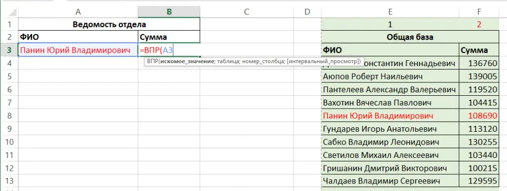
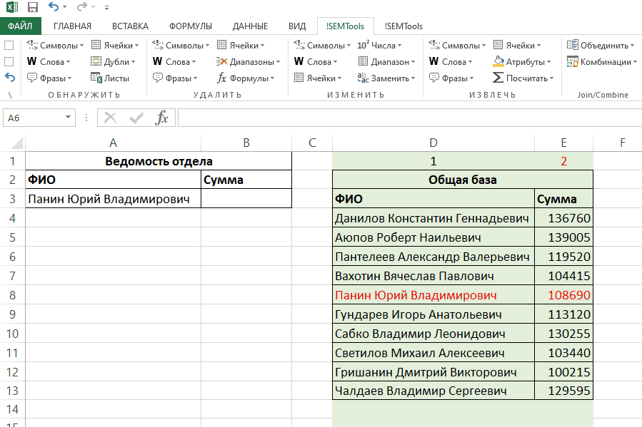
1. What?
What will the formula search for? Typically, this is the address of the cell containing the lookup value.
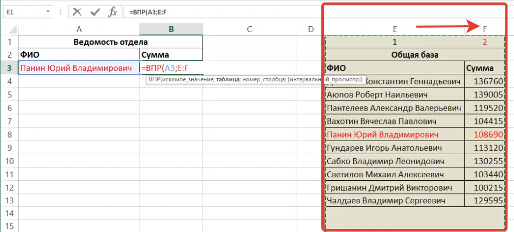
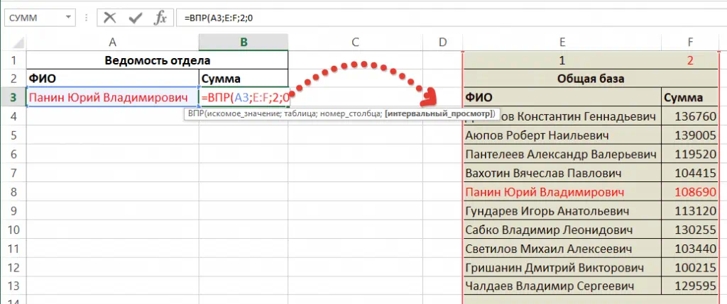
2. Where?
Where will the formula search for the value from step 1? Usually, this is a range of cells consisting of several columns. Tip: Select entire columns (e.g., B:D), not a specific range ($B$2:$D$250). This is faster and doesn’t require anchoring ranges (and you need to anchor them, otherwise when dragging the formula down, the address will change). You can select columns by dragging across the column letters with the left mouse button (as shown by the arrow in the screenshot).
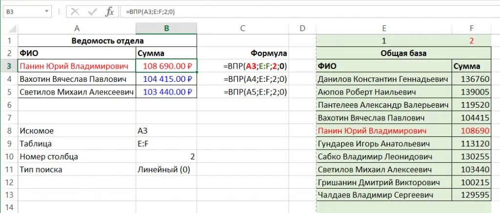
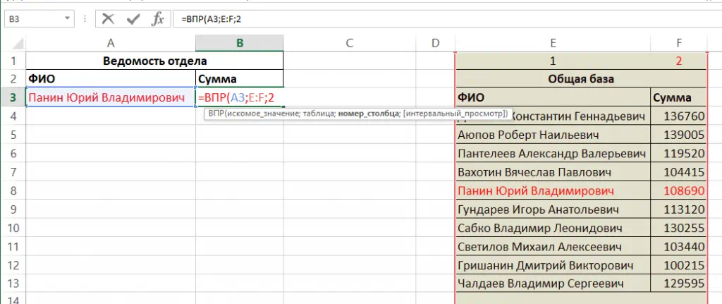
3. When?
When to stop counting from left to right to select the value returned by the formula? In this case, we need the sum, which is the second column of the table.
4. How?
How to search? Read above about the difference in VLOOKUP search methods: Range lookup – 0 or 1, FALSE or TRUE? Usually, linear search is chosen, so enter “0” here.
Just in case, let’s go through all the steps in sequence and see how it looks in practice.
VLOOKUP by partial match
Besides exact match searches, VLOOKUP can also search data with partial matches, as it supports wildcard characters (? and *). Importantly, these are only available in linear search mode (fourth parameter 0 or FALSE). Below is an example using the question mark, which represents any single character:
VLOOKUP not working – errors and causes
The VLOOKUP function sometimes behaves unpredictably – for example, it doesn’t return values, returns errors where it shouldn’t, or returns unexpected values. Let’s examine why VLOOKUP might not work as expected.
VLOOKUP returns #N/A error
VLOOKUP formulas return “#N/A” error when the function cannot find the lookup value in the specified table. Understand that the search is performed only in the first column, and also – if you don’t anchor the search range, it will shift when dragging the formula down, which in 99% of cases will cause errors.
Want to get rid of the error when the lookup value isn’t found? Read how to do this using the IFERROR function in the corresponding article. I’ll just provide the formulas from there:
Text “error” if error occurs:
=IFERROR(VLOOKUP(lookup_value, table_array, col_index_num, 0), "error")
Or empty if error (cell will be blank):
=IFERROR(VLOOKUP(lookup_value, table_array, col_index_num, 0), "")
VLOOKUP doesn’t return value even though lookup exists in table
Sometimes this happens – you can see the data you’re looking for in the table, but VLOOKUP seems to not work. It doesn’t find the data. The problem is always with the data itself, not VLOOKUP, and they really don’t match. The most common problems when cells appear identical visually but actually aren’t:
- Extra spaces in the lookup values or search range that need to be removed
- Non-breaking spaces are used in cells instead of regular spaces – visually there’s no difference, but the program sees it
- Data contains line breaks, tab characters, carriage returns and other types of “invisible” characters
- Cyrillic characters are used instead of Latin or vice versa for letters with identical appearance (to the computer, Russian A and English A are different characters!). Then you need to replace Cyrillic with similar Latin characters (or vice versa)
- Numbers formatted as text, or vice versa
- Different data types between lookup value and table data
The recommendation in such cases is: Try comparing the cells that appear identical separately (For example, copy them to cells A1 and A2 on another sheet). First compare them entirely (=A1=A2, should return “TRUE”), if it returns “FALSE”, compare them character by character (first character with first, second with second, etc.), the MID function can help you here.
Like the article? Help its author! Buy !SEMTools, it has lots of useful instruments to process text data.